Quantile Treatment Effects
The objective of this workbook is to work through estimation of quantile treatment effects using the Lalonde experimental and observational data.
Description of Data
Our example data will be drawn from the infamous Lalonde study:
- Robert Lalonde, “Evaluating the Econometric Evaluations of Training Programs”, American Economic Review, Vol. 76, pp. 604-620
From Dehejia and Wahba (1999):
Lalonde estimated the impact of the National Supported Work (NSW) Demonstration, a labor training program, on postintervention income levels. He used data from a randomized evaluation of the program and examined the extent to which nonexperimental estimators can replicate the unbiased experimental estimate of the treatment impact when applied to a composite dataset of experimental treatment units and nonexperimental comparison units.
Explore Data
Experimental Data
lalonde.exp %>%
  group_by(treat) %>%
skim()| Name | Piped data |
| Number of rows | 445 |
| Number of columns | 13 |
| _______________________ | |
| Column type frequency: | |
| numeric | 12 |
| ________________________ | |
| Group variables | treat |
Variable type: numeric
| skim_variable | treat | n_missing | complete_rate | mean | sd | p0 | p25 | p50 | p75 | p100 | hist |
|---|---|---|---|---|---|---|---|---|---|---|---|
| age | 0 | 0 | 1 | 25.05 | 7.06 | 17 | 19.00 | 24.0 | 28.00 | 55 | ▇▅▂▁▁ |
| age | 1 | 0 | 1 | 25.82 | 7.16 | 17 | 20.00 | 25.0 | 29.00 | 48 | ▇▇▂▁▁ |
| education | 0 | 0 | 1 | 10.09 | 1.61 | 3 | 9.00 | 10.0 | 11.00 | 14 | ▁▁▃▇▂ |
| education | 1 | 0 | 1 | 10.35 | 2.01 | 4 | 9.00 | 11.0 | 12.00 | 16 | ▁▂▇▃▁ |
| black | 0 | 0 | 1 | 0.83 | 0.38 | 0 | 1.00 | 1.0 | 1.00 | 1 | ▂▁▁▁▇ |
| black | 1 | 0 | 1 | 0.84 | 0.36 | 0 | 1.00 | 1.0 | 1.00 | 1 | ▂▁▁▁▇ |
| hispanic | 0 | 0 | 1 | 0.11 | 0.31 | 0 | 0.00 | 0.0 | 0.00 | 1 | ▇▁▁▁▁ |
| hispanic | 1 | 0 | 1 | 0.06 | 0.24 | 0 | 0.00 | 0.0 | 0.00 | 1 | ▇▁▁▁▁ |
| married | 0 | 0 | 1 | 0.15 | 0.36 | 0 | 0.00 | 0.0 | 0.00 | 1 | ▇▁▁▁▂ |
| married | 1 | 0 | 1 | 0.19 | 0.39 | 0 | 0.00 | 0.0 | 0.00 | 1 | ▇▁▁▁▂ |
| nodegree | 0 | 0 | 1 | 0.83 | 0.37 | 0 | 1.00 | 1.0 | 1.00 | 1 | ▂▁▁▁▇ |
| nodegree | 1 | 0 | 1 | 0.71 | 0.46 | 0 | 0.00 | 1.0 | 1.00 | 1 | ▃▁▁▁▇ |
| re74 | 0 | 0 | 1 | 2107.03 | 5687.91 | 0 | 0.00 | 0.0 | 139.42 | 39571 | ▇▁▁▁▁ |
| re74 | 1 | 0 | 1 | 2095.57 | 4886.62 | 0 | 0.00 | 0.0 | 1291.47 | 35040 | ▇▁▁▁▁ |
| re75 | 0 | 0 | 1 | 1266.91 | 3102.98 | 0 | 0.00 | 0.0 | 650.10 | 23032 | ▇▁▁▁▁ |
| re75 | 1 | 0 | 1 | 1532.06 | 3219.25 | 0 | 0.00 | 0.0 | 1817.28 | 25142 | ▇▁▁▁▁ |
| re78 | 0 | 0 | 1 | 4554.80 | 5483.84 | 0 | 0.00 | 3138.8 | 7288.42 | 39484 | ▇▂▁▁▁ |
| re78 | 1 | 0 | 1 | 6349.15 | 7867.40 | 0 | 485.23 | 4232.3 | 9643.00 | 60308 | ▇▁▁▁▁ |
| u74 | 0 | 0 | 1 | 0.75 | 0.43 | 0 | 0.75 | 1.0 | 1.00 | 1 | ▂▁▁▁▇ |
| u74 | 1 | 0 | 1 | 0.71 | 0.46 | 0 | 0.00 | 1.0 | 1.00 | 1 | ▃▁▁▁▇ |
| u75 | 0 | 0 | 1 | 0.68 | 0.47 | 0 | 0.00 | 1.0 | 1.00 | 1 | ▃▁▁▁▇ |
| u75 | 1 | 0 | 1 | 0.60 | 0.49 | 0 | 0.00 | 1.0 | 1.00 | 1 | ▅▁▁▁▇ |
| id | 0 | 0 | 1 | 315.50 | 75.20 | 186 | 250.75 | 315.5 | 380.25 | 445 | ▇▇▇▇▇ |
| id | 1 | 0 | 1 | 93.00 | 53.55 | 1 | 47.00 | 93.0 | 139.00 | 185 | ▇▇▇▇▇ |
Observational (Panel) Data from the Panel Survey of Income Dynamics
lalonde.psid.panel %>%
  group_by(treat) %>%
skim()| Name | Piped data |
| Number of rows | 8025 |
| Number of columns | 13 |
| _______________________ | |
| Column type frequency: | |
| character | 1 |
| numeric | 11 |
| ________________________ | |
| Group variables | treat |
Variable type: character
| skim_variable | treat | n_missing | complete_rate | min | max | empty | n_unique | whitespace |
|---|---|---|---|---|---|---|---|---|
| uniqueid | 0 | 0 | 1 | 8 | 10 | 0 | 7470 | 0 |
| uniqueid | 1 | 0 | 1 | 6 | 8 | 0 | 555 | 0 |
Variable type: numeric
| skim_variable | treat | n_missing | complete_rate | mean | sd | p0 | p25 | p50 | p75 | p100 | hist |
|---|---|---|---|---|---|---|---|---|---|---|---|
| year | 0 | 0 | 1 | 1975.67 | 1.70 | 1974 | 1974 | 1975.0 | 1978.0 | 1978 | ▇▇▁▁▇ |
| year | 1 | 0 | 1 | 1975.67 | 1.70 | 1974 | 1974 | 1975.0 | 1978.0 | 1978 | ▇▇▁▁▇ |
| id | 0 | 0 | 1 | 2035.05 | 2876.75 | 186 | 808 | 1430.5 | 2053.0 | 23100 | ▇▁▁▁▁ |
| id | 1 | 0 | 1 | 93.00 | 53.45 | 1 | 47 | 93.0 | 139.0 | 185 | ▇▇▇▇▇ |
| re | 0 | 0 | 1 | 20015.33 | 14260.04 | 0 | 10742 | 19210.5 | 27337.9 | 156653 | ▇▂▁▁▁ |
| re | 1 | 0 | 1 | 3325.59 | 6046.71 | 0 | 0 | 0.0 | 4574.5 | 60308 | ▇▁▁▁▁ |
| age | 0 | 0 | 1 | 34.85 | 10.44 | 18 | 26 | 33.0 | 44.0 | 55 | ▇▇▆▅▅ |
| age | 1 | 0 | 1 | 25.82 | 7.14 | 17 | 20 | 25.0 | 29.0 | 48 | ▇▇▂▁▁ |
| education | 0 | 0 | 1 | 12.12 | 3.08 | 0 | 11 | 12.0 | 14.0 | 17 | ▁▁▃▇▅ |
| education | 1 | 0 | 1 | 10.35 | 2.01 | 4 | 9 | 11.0 | 12.0 | 16 | ▁▂▇▃▁ |
| black | 0 | 0 | 1 | 0.25 | 0.43 | 0 | 0 | 0.0 | 1.0 | 1 | ▇▁▁▁▃ |
| black | 1 | 0 | 1 | 0.84 | 0.36 | 0 | 1 | 1.0 | 1.0 | 1 | ▂▁▁▁▇ |
| hispanic | 0 | 0 | 1 | 0.03 | 0.18 | 0 | 0 | 0.0 | 0.0 | 1 | ▇▁▁▁▁ |
| hispanic | 1 | 0 | 1 | 0.06 | 0.24 | 0 | 0 | 0.0 | 0.0 | 1 | ▇▁▁▁▁ |
| married | 0 | 0 | 1 | 0.87 | 0.34 | 0 | 1 | 1.0 | 1.0 | 1 | ▁▁▁▁▇ |
| married | 1 | 0 | 1 | 0.19 | 0.39 | 0 | 0 | 0.0 | 0.0 | 1 | ▇▁▁▁▂ |
| nodegree | 0 | 0 | 1 | 0.31 | 0.46 | 0 | 0 | 0.0 | 1.0 | 1 | ▇▁▁▁▃ |
| nodegree | 1 | 0 | 1 | 0.71 | 0.46 | 0 | 0 | 1.0 | 1.0 | 1 | ▃▁▁▁▇ |
| u74 | 0 | 0 | 1 | 0.09 | 0.28 | 0 | 0 | 0.0 | 0.0 | 1 | ▇▁▁▁▁ |
| u74 | 1 | 0 | 1 | 0.71 | 0.46 | 0 | 0 | 1.0 | 1.0 | 1 | ▃▁▁▁▇ |
| u75 | 0 | 0 | 1 | 0.10 | 0.30 | 0 | 0 | 0.0 | 0.0 | 1 | ▇▁▁▁▁ |
| u75 | 1 | 0 | 1 | 0.60 | 0.49 | 0 | 0 | 1.0 | 1.0 | 1 | ▅▁▁▁▇ |
A key takeaway is that the experimental data is reasonably balanced across treated and control units (not surprisingly) but the observational data is not.
Evaluate the Job Training Program
Quantile Treatment Effect Estimation in Experimental Data
Our first exercise will evaluate the effect of the training program using the experimental data. Because we have a randomized experiment, we can simply compare the treated and untreated outcomes in the post-treatment period.
Let’s first take a look at the distribution of outcomes by group:
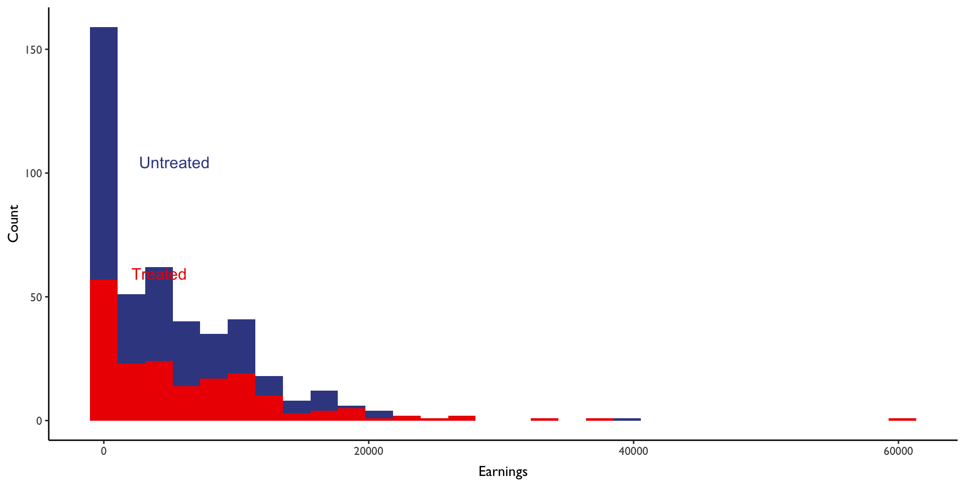
We next take a difference in means to obtain an estimate of the average treatment effect on the treated:
lalonde.exp %>%
  group_by(treat) %>%
  summarise(mean_outcome = mean(re78)) %>%
  mutate(att = mean_outcome - lag(mean_outcome)) %>%
kable(digits = 2) %>% kable_styling()| treat | mean_outcome | att |
|---|---|---|
| 0 | 4554.8 | NA |
| 1 | 6349.1 | 1794.3 |
Suppose we wanted to estimate treatment effects at different quantiles of the outcome distribution. To get a sense of where these effects may occur, we can plot the empirical cumulative distribution function (eCDF) for each group:
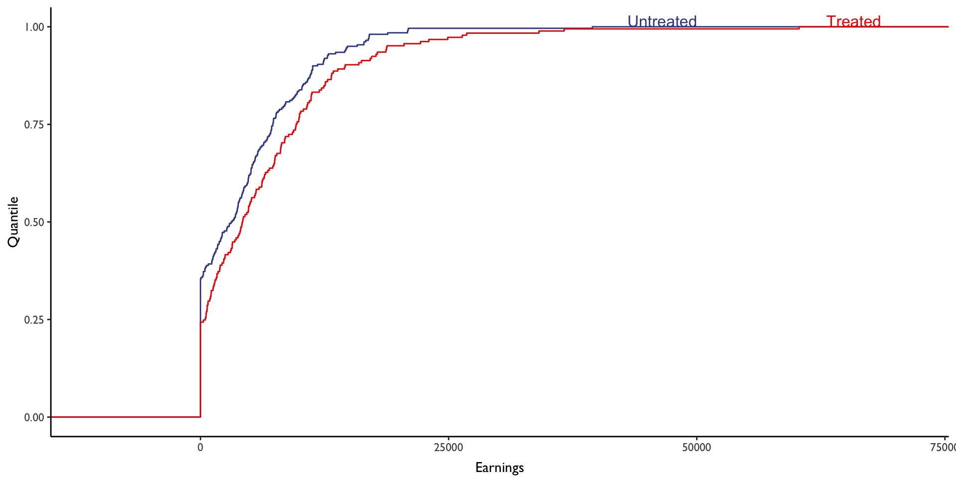
We see here that the two distributions have separated a bit, though there are regions where they essentially overlap. Just shy of the 25th percentile, for example, the two distributions overlap at around $0 in income; there doesn’t appear to be any change in earnings for treated individuals within the bottom quarter of the income distribution.
Estimating Quantile Treatment Effects
Suppose we wanted to estimate the difference at some quantile of interest (e.g., the 25th percentile or the 75th percentile). How would we go about doing this? Essentially, for a selected quantile (e.g., 75th percentile), we need to measure the horizontal distance between the two curves in Figure 2.
To build up an estimator that we can apply in our data, we first need to introduce some notation.
Define \(F_{Y(W)wt}(y)\) as the potential outcome distribution function for an individual receiving treatment \(W \in 0,1\), and who is observed to be in treatment group \(w\) at time \(t\).
For example:
- \(F_{Y(1)11}(y)\) is the distribution function for the outcome distribution under treatment for treated individuals in the post-treatment period.
- \(F_{Y(0)01}(y)\) is the distribution function for the outcome distribution under non-treatment for non-treated individuals in the post-treatment period.
We can supply each of these distribution functions a value of the outcome \(y\), and it will tell us at what quantile \(\tau\) in the distribution that value of \(y\) maps to. For example, plugging in a value of $2,000 might tell us that this value is at the 50th percentile (median) of a given outcome distribution.
Stepping back from the notation a bit, note that these two functions are essentially what we already plotted in Figure 2 above. How do we calculate these functions in R?
Fortunately, base R has a defined function (ecdf()) that allows us to do this easily. Let’s define empirical distribution functions for the treated and untreated groups in the experimental Lalonde data:
y11 <- lalonde.exp %>% filter(treat==1) %>% pull(re78)
y01 <- lalonde.exp %>% filter(treat==0) %>% pull(re78)

eF11 <- ecdf(y11)
eF01 <- ecdf(y01)

eF11(2000)
[1] 0.38919eF01(2000)[1] 0.45We see in the calculations above that earnings of $2,000 would place you at the 39th percentile of the treated group’s post-intervention outcome distribution, and at the 45th percentile of the untreated groups distribution.
We next need to go one step further, however, and define the inverse of the above. That is, we need a function that, provided a quantile value \(\tau\), returns the outcome value that maps to that quantile in the distribution. This is fundamentally what we’ll be working with to estimate treatment effects because we want to know what the effect of the program is at the 75th percentile, not for someone with $2,000 in earnings.
The concept described above is known as the inverse distribution function, and in our notation will be defined as \(F^{-1}_{Y(W)wt}(\tau)\). That is, we supply this function with a quantile \(\tau\), and it returns the value associated with the outcome distribution at that particular quantile.
From a practical sense, calculating the inverse CDF in R is straightforward, however there is not a base function like ecdf() we can draw from. Fortunately, the package edfun provides us with an easy way to calculate it.
invF11 <- edfun::edfun(y11)$qfun
invF01 <- edfun::edfun(y01)$qfun

invF11(0.75)
[1] 9631.9invF01(0.75)[1] 7284.4In the calculated values above, an earnings value of 9632 would place you at the 75th percentile of the treated group’s post-intervention outcome distribution. Similarly, an earnings value of 7284 would place you at the 75th percentile of the untreated group’s post-intervention outcome distribution.
We’re now ready to estimate quantile treatment effects. Formally, the quantile treatment effect on the treated (QTT) at \(\tau\) is obtained as the difference in the inverse distribution function for the treated group in the post period under treatment and under non-treatment:
\[ \Delta_{\tau} = F^{-1}_{Y(1)11}(\tau) - F^{-1}_{Y(0)11}(\tau) \]
However, as usual the second quantity is an unobserved counterfactual. Given random assignment, we can estimate QTTs using the inverse distribution function from the untreated group.
\[ \Delta_{\tau} = F^{-1}_{Y(1)11}(\tau) - F^{-1}_{Y(0)01}(\tau) \]
So what is QTT(0.75) in the Lalonde experimental data?
invF11(0.75) - invF01(0.75)[1] 2347.5There it is; we’ve calculated a quantile treatment effect in our experimental data!
In practice we do not need to go through the above process by hand each time. We can actually just plug our data into the qte package’s functions to obtain estimates and standard errors:
att_experimental <-
  ci.qtet(re78 ~ treat,
    data=lalonde.exp,
    probs=seq(0.05,0.95,0.05),
    se=T,
    iters=10)
res_att_experimental <- summary(att_experimental)
Note that the qte package computes standard errors via a bootstrap method.
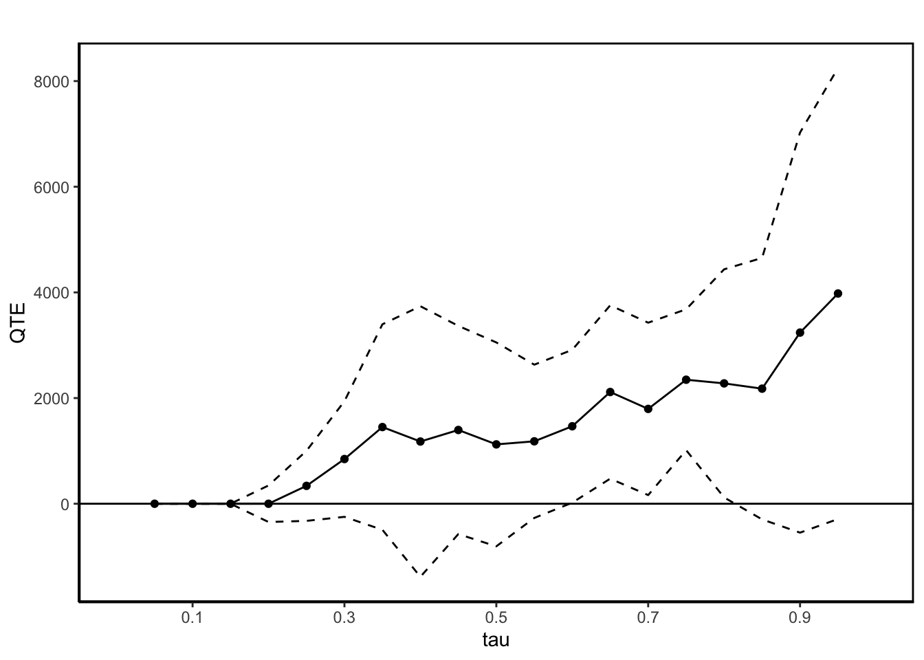
You’ll see in Figure 3 that the estimated QTT for the 75th percentile is exactly the same as we calculated above.
| Percentile | Treatment Effect | Standard Error |
|---|---|---|
| Avg | 1794.3 | 630.2 |
| 95% | 3979.6 | 2177.9 |
| 90% | 3239.6 | 1932.0 |
| 85% | 2178.3 | 1262.6 |
| 80% | 2278.1 | 1101.5 |
| 75% | 2347.5 | 680.2 |
| 70% | 1795.1 | 832.4 |
| 65% | 2115.0 | 836.9 |
| 60% | 1466.5 | 737.9 |
| 55% | 1181.5 | 740.2 |
| 50% | 1123.5 | 984.5 |
| 45% | 1396.1 | 1005.2 |
| 40% | 1177.7 | 1306.6 |
| 35% | 1451.5 | 992.3 |
| 30% | 846.4 | 558.3 |
| 25% | 338.6 | 338.2 |
| 20% | 0.0 | 176.4 |
| 15% | 0.0 | 0.0 |
| 10% | 0.0 | 0.0 |
| 5% | 0.0 | 0.0 |
Quantile Treatment Effect Estimation in Observational Data
Now suppose we do not have the luxury of experimental data, but instead have a treated group and untreated group drawn from observational data. How can we identify and estimate quantile treatment effects?
There are a number of approaches we can take here:
- Estimate bounds on the quantile treatment effect distribution.
- Estimate QTTs under an assumption of conditional independence, i.e., unconfoudnendess.
- Estimate QTTs using a quantile difference-in-differences (qDID) estimator.
- Estimate QTTs using a changes-in-changes (CiC) estimator (Athey and Imbens 2006).
Partial identification via estimating bounds (#1) will be a focus of our class next week, so we’ll set it aside for now – though note that the qte package can estimate bounds based on the method in Fan and Yu (2012).
Similarly, if we think we have enough measured data satisfy an unconfoundedness assumption (analogous to what we do with propensity scores ore matching) we can also estimate (#2) using the qte package.
Our focus for today will be on approaches (#3) and especially (#4). We’ll also discuss how we can incorporate covariates to improve identifcation of quantile treatment effects.
Intuition for qDID and CiC
Essentially, we’re going to lean on similar intuition for identifying QTTs as we do for identifying average treatment effects on the treated using difference-in-differences. In the case of quantile effects, however, we will be thinking in terms of how the distribution functions change in an untreated comparison group. We’ll then use these changes as a “stand-in” for the counterfactual change that would have occurred in the treated group absent the treatment.
The difference between qDID and CiC essentially boils down to how we think about the counterfactual. Let’s envision two scenarios with observational data for a job training program under which the treatment group is selected predominantly among unemployed individuals with low earnings:
The pre-intervention earnings at the 50th percentile in the treatment group are $0, and at the 50th percentile of the untreated group, pre-intervention earnings are $5,000. In the post-intervention period, the untreated group’s earnings increase to $6,000 at the 50th percentile, while the treated group’s earnings rise to $3000 at the 50th percentile.
The pre-intervention earnings at the 50th percentile in the treatment group are $0, and $0 in earnings corresponds to the 10th percentile of the untreated group’s pre-intervention earnings distribution. In the post period, the untreated group’s earnings remain at $0 at the 10th percentile, while earnings at the 50th percentile in the treated group rise to $3,000.
What counterfactual should we use for the treated group? The $1,000 rise in earnings observed at the 50th percentile in the untreated group, even though the baseline value at the 50th percentile was very different than the treated group’s median value? Or, is a better estimate of the counterfactual the experience of $0 earners at the 10th percentile in the untreated group? In short, the former assumption is used for qDID, while the latter assumption is used for CiC.
Estimating qDID and CiC
With the intuition for both approaches solidified, let’s now construct quantile treatment effect estimates in the observational Lalonde data using each.
First, let’s pull out the outcome values for treated and control groups in the pre (1975) and post-intervention (1978) periods:
y00 <- lalonde.psid %>%
  filter(treat==0) %>%
  pull(re75)

y10 <- lalonde.psid %>%
  filter(treat==1) %>%
  pull(re75)

y01 <- lalonde.psid %>%
  filter(treat==0) %>%
  pull(re78)

y11 <- lalonde.psid %>%
  filter(treat==1) %>%
  pull(re78)
We’ll next define eCDFs and inverse eCDFs for each:
eF00 <- ecdf(y00)
invF00 <- edfun::edfun(y00)$qfun

eF10 <- ecdf(y10)
invF10 <- edfun::edfun(y10)$qfun

eF01 <- ecdf(y01)
invF01 <- edfun::edfun(y01)$qfun

eF11 <- ecdf(y11)
invF11 <- edfun::edfun(y11)$qfun
The next thing we need to do is to define a quantile of interest. Let’s estimate for the 75th percentile.
q = 0.75Next, let’s estimate the observed change in the treated group at the 75th percentile:
invF11(q)[1] 9631.9invF10(q)[1] 1809change_treated <- invF11(q) - invF10(q)
change_treated[1] 7822.9So we observe earnings going up by 7823. But what would have happened counterfactually? For this we will appeal to the untreated group’s experience.
First, let’s estimate what change happens at the 75th percentile of the untreated group’s earnings distribution:
invF01(q)[1] 29510invF00(q)[1] 26470cfx_untreated_q75 <- invF01(q) - invF00(q)
cfx_untreated_q75 [1] 3040.2To construct a qDID estimate, we’d simply net out this counterfactual from the observed change in the treated group:
qtt_qDID <- change_treated - cfx_untreated_q75
qtt_qDID
[1] 4782.7Using qDID, we would estimate that the job trainings program increased earnings by $4783.
Notice, however, that there is a huge difference in earnings at the 75th percentile of the treated group’s pre-intervention earnings distribution ($1809), and the untreated group’s ($26470).
As an alternative, we can adopt a Changes-in-Changes model. Recall from above that this model requires an additional step: we must map the earnings value of the treated group at the 75th percentile to the corresponding quantile in the untreated groups pre-intervention earnings distribution. We then use the change in earnings at this different quantile as an estimate of the counterfactual:
# Earnings at the qth quantile of the treated group
y_q <- invF10(q)
y_q
[1] 1809# Find what quantile this maps to in the untreated group's distribution.
q_star <- eF00(y_q)
q_star[1] 0.11365cfx_CiC <- invF01(q_star) - y_q
cfx_CiC[1] -1809change_treated <- invF11(q) - invF10(q)
change_treated[1] 7822.9qtt_CiC <- change_treated - cfx_CiC
qtt_CiC[1] 9631.9While the above exercises went through estimating a changes-in-changes value by hand, the formal estimator is a bit simpler due to some cancelling out of terms. Specifically, the counterfactual CDF is given by
\[ \hat F_{Y(0),11}(y) = F_{y,01}(F_{y,00}^{-1}(F_{y,10}(y))) \]
where F_{y,00} is the observed CDF for the untreated group in the pre-period, F_{y,10} is the observed CDF for the treated group in the pre period, etc.
Equivalently, we can estimate the inverse CDF of the counterfactual as:
\[ \hat F_{Y(0),11}^{-1}(\tau) = F_{y,01}^{-1}(F_{y,00}(F^{-1}_{y,10}(\tau))) \]
And the treatement effect estimate is given by:
\[ \Delta_{\tau}^{CiC} = F_{Y(1),11}^{-1}(\tau)- \hat F_{Y(0),11}^{-1}(\tau) \]
Implemented for our example, the QTT for the 75th percentile is
invF11(q) - invF01(eF00(invF10(q)))[1] 9631.9which is identical to the “by hand” estimate we calculated above.
Again, the qte package in R will calculate changes-in-changes estimates for you, along with standard errors. The estimates are slightly different here, owing to some “lumpiness” in the eCDFs and slight differnces in calculating the values at quantiles in the data. However, the QTTs are quite close to what we estimated above:
There is also a Stata implementation of the Changes-in-Changes estimator, which can be found here.
df <-
  lalonde.psid %>%
  select(id,re75,re78,treat) %>%
  gather(year,y,-id,-treat) %>%
  tibble() %>%
  mutate(year = ifelse(year=="re75",1975,1978))

est_CiC <- CiC(y ~ treat, t = 1978, tmin1=1975,
               tname = "year", idname = "id",
               data = df, probs = c(q),
               se = TRUE, panel = F)
summary(est_CiC)
Quantile Treatment Effect:

tau QTE Std. Error
0.75    9643.00  973.09

Average Treatment Effect:   5089.64
     Std. Error:        664.74
Changes-in-Changes with Covariates
# Note that this code is simply adapted from the underlying CiC formula to show
# what is going on behind the curtain. Code source: Calloway's qte package.

library(quantreg)
Loading required package: SparseM
Attaching package: 'SparseM'The following object is masked from 'package:base':
backsolve# Quantiles to estimate over
u <- seq(0.01, 0.99, 0.01)
# Extract out various subsets of the data based on treatment and time
df00 = lalonde.psid.panel %>%
filter(treat==0 & year==1975)
df10 = lalonde.psid.panel %>%
filter(treat==1 & year==1975)
df01 = lalonde.psid.panel %>%
filter(treat==0 & year==1978)
df11 = lalonde.psid.panel %>%
filter(treat==1 & year==1978)
# Obtain sample sizes for each subset
n1t <- df11 %>%
nrow()
n1tmin1 <-df10 %>%
nrow()
n0t <- df01 %>%
nrow()
n0tmin1 <- df00 %>%
nrow()
# Quantile regressions of the outcome on covariates
yformla <- "re ~ age + I(age^2) + education + black + hispanic + married + nodegree"
QR0t <- rq(yformla, data = df01 , tau = u)Warning in rq.fit.br(x, y, tau = tau, ...): Solution may be nonuniqueQR0tmin1 <- rq(yformla, data = df00, tau = u)
QR1t <- rq(yformla, data = df11, tau = u)Warning in rq.fit.br(x, y, tau = tau, ...): Solution may be nonunique
Warning in rq.fit.br(x, y, tau = tau, ...): Solution may be nonunique# Obtain predictions of the conditional distribution function given each
# sample individual's covariate
# This is for the pre-period in the control group
QR0tmin1F <- predict(QR0tmin1, newdata = df10,
type = "Fhat", stepfun = TRUE)
# Now map the observed outcome into the quantile of the conditional distribution function
# for each sample individual
F0tmin1 <- sapply(1:n1tmin1, function(i) QR0tmin1F[[i]](df10$re[i]))
QR0tQ <- predict(QR0t, newdata = df10, type = "Qhat",
stepfun = TRUE)
y0t <- sapply(1:n1tmin1, function(i) QR0tQ[[i]](F0tmin1[i]))
F.treatedcf.t <- ecdf(y0t)
att <- mean(df11[, "re"]) - mean(y0t)
q1 = quantile(df11[, "re"], probs = u, type = 1)
q0 = quantile(F.treatedcf.t, probs = u, type = 1)
qte = (q1 - q0); qte 1% 2% 3% 4% 5% 6% 7% 8%
0.00 0.00 0.00 0.00 0.00 0.00 0.00 0.00
9% 10% 11% 12% 13% 14% 15% 16%
0.00 0.00 0.00 0.00 0.00 0.00 0.00 0.00
17% 18% 19% 20% 21% 22% 23% 24%
0.00 0.00 0.00 0.00 0.00 0.00 0.00 0.00
25% 26% 27% 28% 29% 30% 31% 32%
485.23 559.44 590.78 671.33 743.67 929.88 1048.43 1085.44
33% 34% 35% 36% 37% 38% 39% 40%
1294.41 1358.64 1460.36 1652.64 1773.42 1953.27 2164.02 2321.11
41% 42% 43% 44% 45% 46% 47% 48%
2456.15 2787.96 3094.16 3196.57 3462.56 3786.63 3881.28 4032.71
49% 50% 51% 52% 53% 54% 55% 56%
4146.60 4232.31 4321.71 4666.24 4843.18 4849.56 5010.34 5149.50
57% 58% 59% 60% 61% 62% 63% 64%
5522.79 5615.19 6167.68 6181.88 6281.43 6456.70 6788.46 7284.99
65% 66% 67% 68% 69% 70% 71% 72%
7458.11 7506.15 7535.94 8048.60 7461.02 7508.97 7746.03 7953.09
73% 74% 75% 76% 77% 78% 79% 80%
8138.60 8211.33 8210.84 8347.53 8189.37 7911.28 8298.11 8332.69
81% 82% 83% 84% 85% 86% 87% 88%
8164.24 8030.49 7746.49 8426.08 8515.98 8293.94 8147.08 8148.86
89% 90% 91% 92% 93% 94% 95% 96%
8307.59 8822.00 9450.88 9370.33 9691.94 9955.40 8273.74 11024.51
97% 98% 99%
10944.14 12467.26 17466.10 c1 <- CiC(re ~ treat, t=1978, tmin1=1975, tname="year",
xformla=~age + I(age^2) + education + black + hispanic + married + nodegree,
data=lalonde.psid.panel, idname="id", se=FALSE,
probs=seq(0.05, 0.95, 0.05))Warning in rq.fit.br(x, y, tau = tau, ...): Solution may be nonunique
Warning in rq.fit.br(x, y, tau = tau, ...): Solution may be nonunique

Warning in rq.fit.br(x, y, tau = tau, ...): Solution may be nonuniquesummary(c1)
Quantile Treatment Effect:

tau QTE
0.05       0.00
0.1    0.00
0.15       0.00
0.2    0.00
0.25     485.23
0.3  929.88
0.35    1460.36
0.4 2321.11
0.45    3462.56
0.5 4232.31
0.55    5010.34
0.6 6210.67
0.65    7458.11
0.7 7508.97
0.75    8210.84
0.8 8332.69
0.85    8515.98
0.9 8822.00
0.95    8273.74

Average Treatment Effect:   4629.24