Synthetic Control Methods

Motivation

Motivation

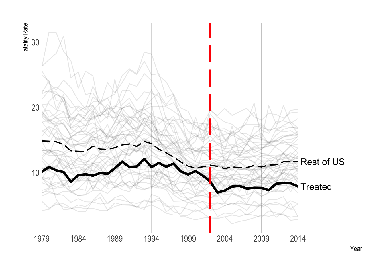
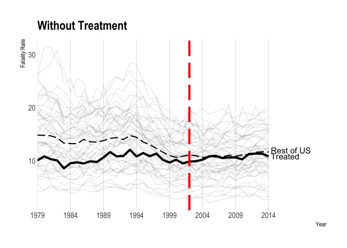
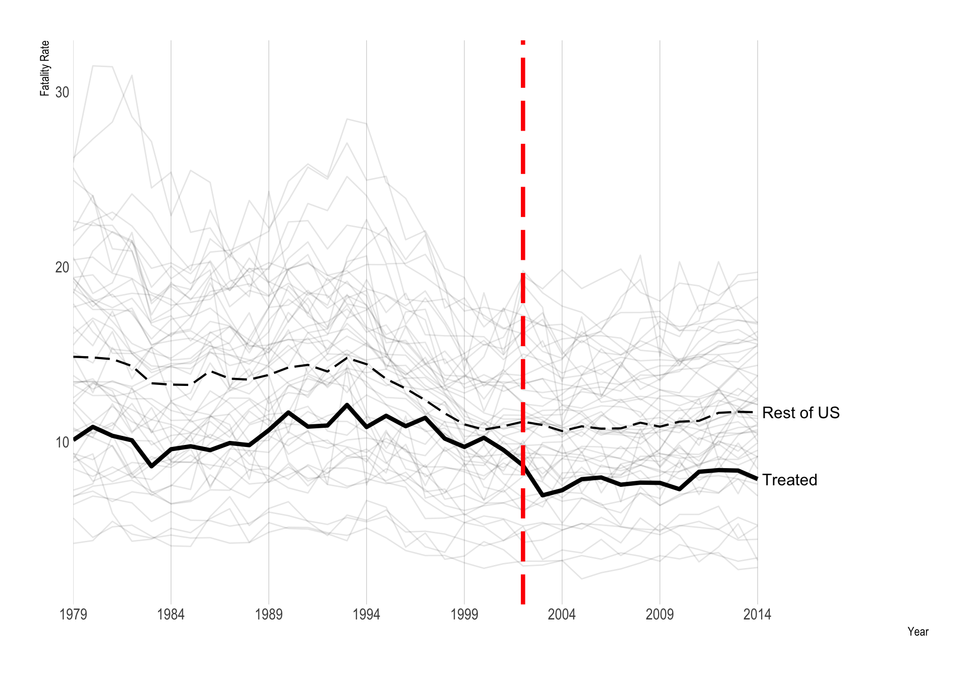
• Hypothetical gun law passed in a single state (Pennsylvania) in 2002.
• The plot shows the total firearm death rate, by year and state
• I have imposed a (simulated) immediately-acting treatment effect (\(\tau = -3\)).

Firearm Death Rate, by State and Year

With Treatment

Without Treatment (True Counterfactual)

How Would You Evaluate This Policy Change?

1. Difference-in-Differences

How Would You Evaluate This Policy Change?

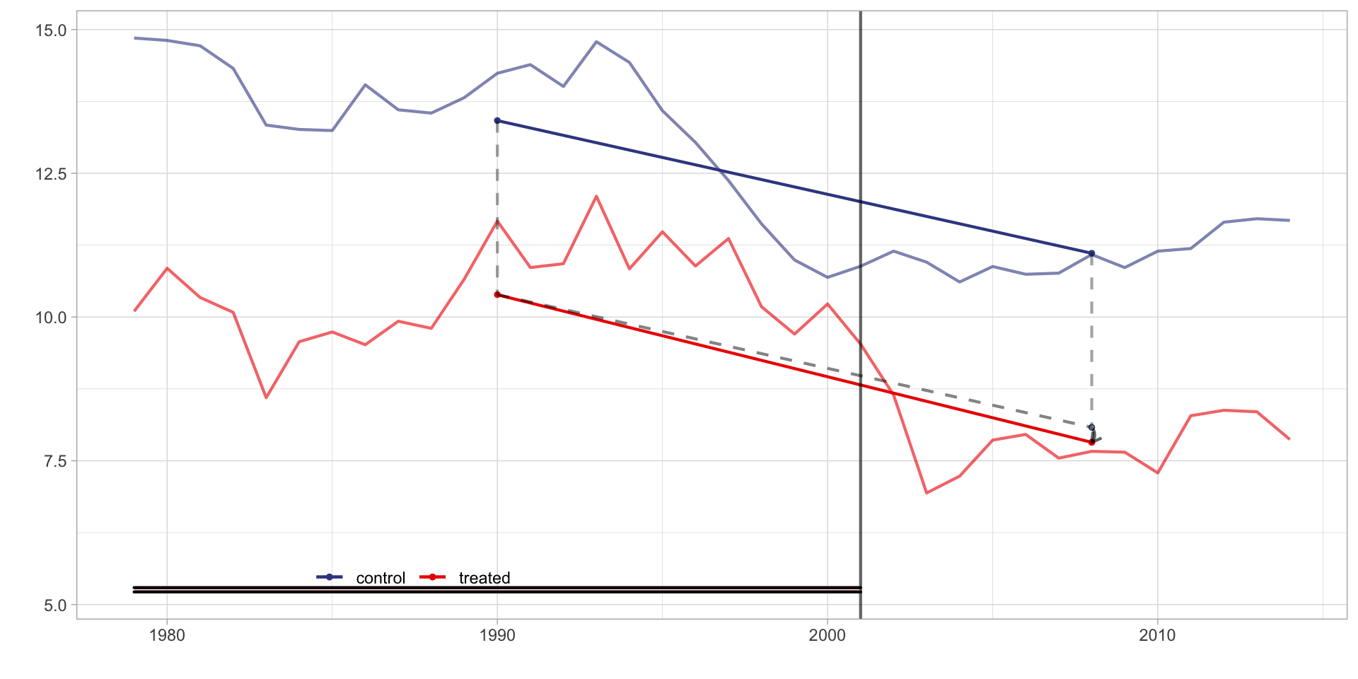
1. Difference-in-Differences
   • Difference in average pre-treatment outcomes between treated and control units is subtracted from the difference in average posttreatment outcomes

How Would You Evaluate This Policy Change?

2. Matching

How Would You Evaluate This Policy Change?

2. Matching
   • For each treated unit, one or more matches are found among the controls, based on both pre-treatment outcomes and other covariates.

How Would You Evaluate This Policy Change?

3. Synthetic control

How Would You Evaluate This Policy Change?

3. Synthetic control
   • For each treated unit, a synthetic control is constructed as a weighted average of control units that matches pretreatment outcomes and covariates for the treated units.

How Would You Evaluate This Policy Change?

4. Regression methods (e.g., interrupted time series, imputation estimators)

How Would You Evaluate This Policy Change?

4. Regression methods (e.g., interrupted time series, imputation estimators)
   • Post-treatment outcomes for control units are regressed on pre-treatment outcomes and other covariates and the regression coefficients are used to predict the counterfactual outcome for the treated units.

A Generalized Framework

• \(N + 1\) units observed for \(T\) periods, with a subset of treated units (for simplicity - unit 0) treated from \(T0\) onwards.

• Time-varying treatment indicator: \(W_{i,t}\)

• Potential outcomes for unit \(0\) define the treatment effect: \(\tau_{0,t} := Y_{0,t}(1) − Y_{0,t}(0)\) for \(t = T0 + 1, . . . , T\)

A Generalized Framework

• Observed outcome: \(Y^{obs}_{i,t} = Y_{i,t}(W_{i,t})\)

• Time-invariant characteristics \(X_i := (X_{i,1}, . . . , X_{i,M} )^T\) for each unit, which may include lagged outcomes Y^{obs}_{i,t} for \(t ≤ T0\).

Data Setup

state	year	deaths	population	crude_rate	crude_rate_lag1	crude_rate_lag2	crude_rate_lag3	year_cat	pc1	pc2	pc3	pc4	pc5	pc6	pc7	pc8	pc9	pc10	pc11	pc12	pc13	pc14	pc15	pc16	pc17	pc18	pc19	pc20	pc21	pc22	pc23	pc24	pc25	pc26	pc27	pc28	pc29	pc30	pc31	pc32	population_std	levels_coding	ch_levels_coding	cr_adj	cr_adj_lag1	lag1
Alabama	1979	856	3873403	22.10	NA	NA	NA	1979	-3.05	3.15	2.02	-0.10	-0.63	-0.36	-0.04	0.13	0.03	0.19	0.31	-0.14	0.36	-0.24	-0.64	-0.85	0.24	-0.17	0.15	0.05	-0.45	-0.05	0.11	-0.17	0.32	0.10	0.09	-0.03	0.05	0.06	-0.04	-0.02	0.72	0	0	22.10	NA	NA
Alabama	1980	938	3898117	24.06	22.10	NA	NA	1980	-3.47	3.49	2.05	-0.10	-0.53	-0.34	0.26	0.39	-0.01	0.61	0.03	0.11	0.05	-0.20	-0.81	-1.10	0.38	0.23	0.00	0.49	-0.94	0.05	0.19	-0.19	0.01	0.38	-0.08	-0.07	-0.06	0.20	-0.05	-0.07	0.72	0	0	24.06	22.10	22.10
Alabama	1981	824	3920097	21.02	24.06	22.10	NA	1981	-3.42	3.56	2.27	-0.50	-0.50	-0.70	0.20	0.33	0.20	0.39	-0.01	0.07	0.18	-0.63	-0.85	-0.69	0.34	0.27	0.17	0.49	-0.43	0.08	0.16	-0.28	0.26	0.28	-0.12	0.02	-0.01	0.14	-0.03	-0.04	0.72	0	0	21.02	24.06	24.06
Alabama	1982	820	3925924	20.89	21.02	24.06	22.10	1982	-3.23	3.35	2.07	-0.45	-0.53	-1.09	0.04	0.50	0.45	0.26	0.48	0.11	-0.04	-0.57	-0.12	-0.24	0.15	-0.04	0.22	0.07	-0.25	0.38	-0.06	-0.38	0.03	-0.19	0.00	0.11	0.06	0.02	0.06	-0.02	0.73	0	0	20.89	21.02	21.02
Alabama	1983	710	3933838	18.05	20.89	21.02	24.06	1983	-3.06	3.41	1.92	-0.49	-0.37	-0.75	0.48	0.43	-0.10	0.20	0.29	0.14	0.00	-1.14	-0.73	-0.26	0.19	0.17	0.32	0.11	-0.18	0.53	0.01	-0.22	0.05	0.10	0.05	0.27	0.11	-0.01	0.04	0.00	0.73	0	0	18.05	20.89	20.89
Alabama	1984	750	3952400	18.98	18.05	20.89	21.02	1984	-2.62	3.24	1.44	-0.31	-0.23	-0.49	0.79	0.56	-0.27	0.41	0.31	0.12	-0.21	-1.26	-0.69	-0.09	0.01	-0.07	0.13	0.02	-0.18	0.44	-0.16	-0.34	-0.02	0.09	-0.10	0.23	-0.02	0.04	0.14	0.03	0.73	0	0	18.98	18.05	18.05

A Generalized Framework

• Let’s focus on the last period:

\[ \tau_{0,T} = Y_{0,T}(1) − Y_{0,T}(0) = Y^{obs}_{0,T} − \color{red}{Y_{0,T}(0)} \] - The last (red) value is an unobserved counterfactual.

A Generalized Framework

• The above methods impute \(Y_{0,T}(1)\) with a linear structure: \[ \hat{Y}_{0,T}(0) = \mu + \sum_{i=1}^n \omega_i \cdot Y^{obs}_{i,T} \]
• The methods differ in whether and how they choose \(\mu\) and \(\omega_i\) given the observed data.

A Menu of Constraints

1. No Intercept: \(\mu = 0\)
2. Adding Up: \(\sum_{i=1}^{n} \omega_i = 1\)
3. Non-negativity: \(\omega_i >= 0\) for all \(i\)
4. Constant weights: \(\omega_i = \bar \omega\) for all \(i\).

1. No Intercept: \(\mu = 0\)

• Rules out the possibility that the outcome for the treated unit is systematically different, by a constant amount, than the other units.
• A hallmark of difference-in-differences is that the outcome levels can vary by a fixed difference over time as long as parallel trends holds.

2. Adding Up: \(\sum_{i=1}^{n} \omega_i = 1\)

• Requires that the weights sum up to one.
• Common in matching strategies.
• Implausible if the treated unit is an outlier relative to other units.
• Combined with constraint #1, it may be difficult to obtain good predictions for extreme units.

2. Adding Up: \(\sum_{i=1}^{n} \omega_i = 1\)

Hollingsworth and Wing (2022)

3. Non-negativity: \(\omega_i >= 0\) for all \(i\)

• Is an important restriction on standard synthetic control methods.
• Helps ensure that there is a unique solution for control unit weights.
• Often ensures that the weights are non-zero only for a small subset of the control units, making the weights easier to interpret.

4. Constant weights: \(\omega_i = \bar \omega\) for all \(i\).

• Strengthens the nonnegativity condition by making the assumption that all control units are equally valid.
• Common in DID (we’ll see this in a minute).
• In conjuction to constraint 2 (Adding Up), implies that weights are all equal to 1/N, where N is number of control units.

Difference-in-differences (DID)

Difference-in-Differences

1. No Intercept: \(\mu = 0\)

2. Adding Up: \(\sum_{i=1}^{n} \omega_i = 1\)

3. Non-negativity: \(\omega_i >= 0\) for all \(i\)

4. Constant weights: \(\omega_i = \bar \omega\) for all \(i\).

Difference-in-Differences

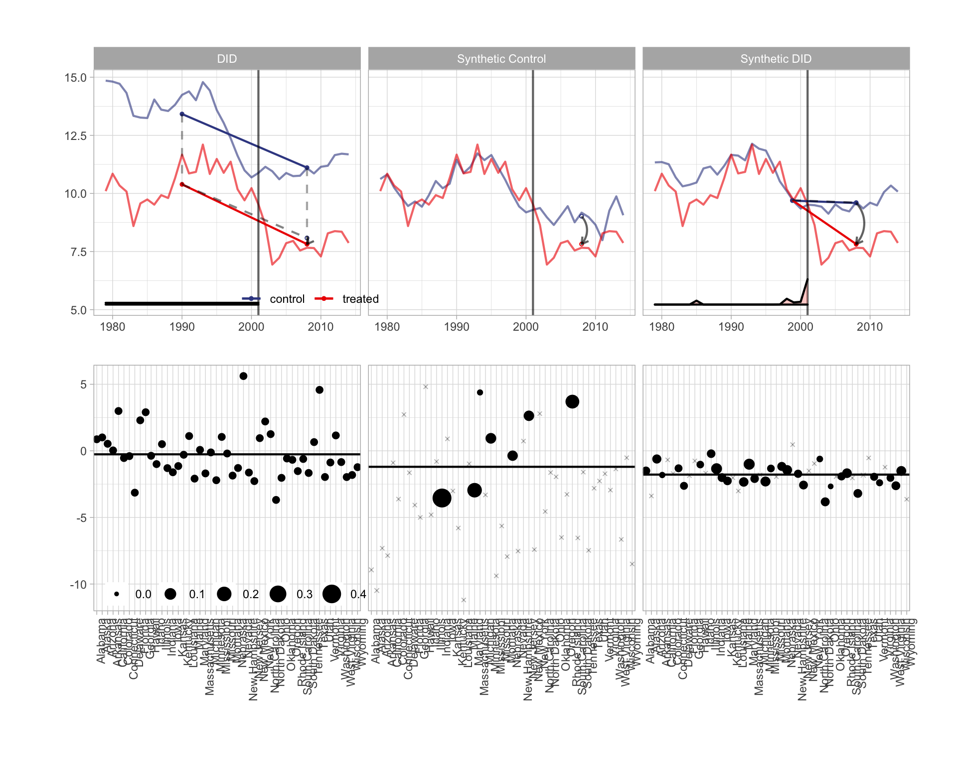
Total Firearm Death Rate, by Year and State

Difference-in-Differences Estimate

\(\hat \tau\) = -0.261

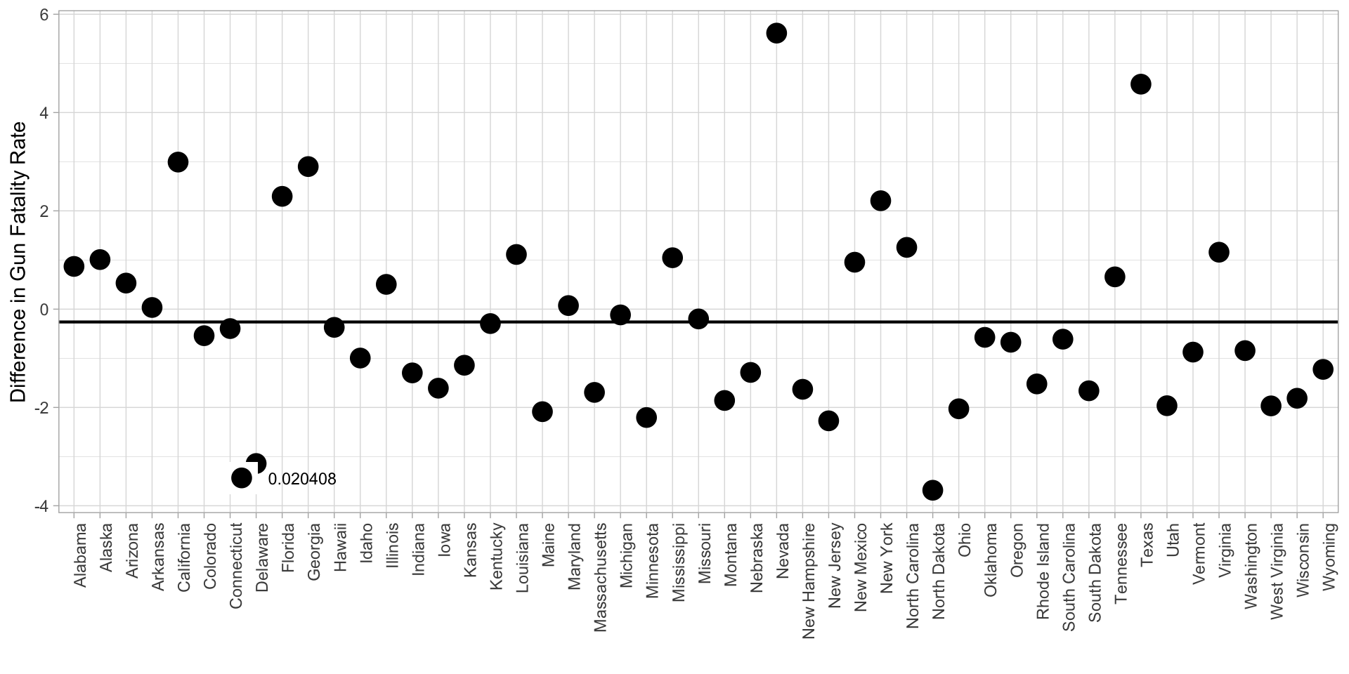
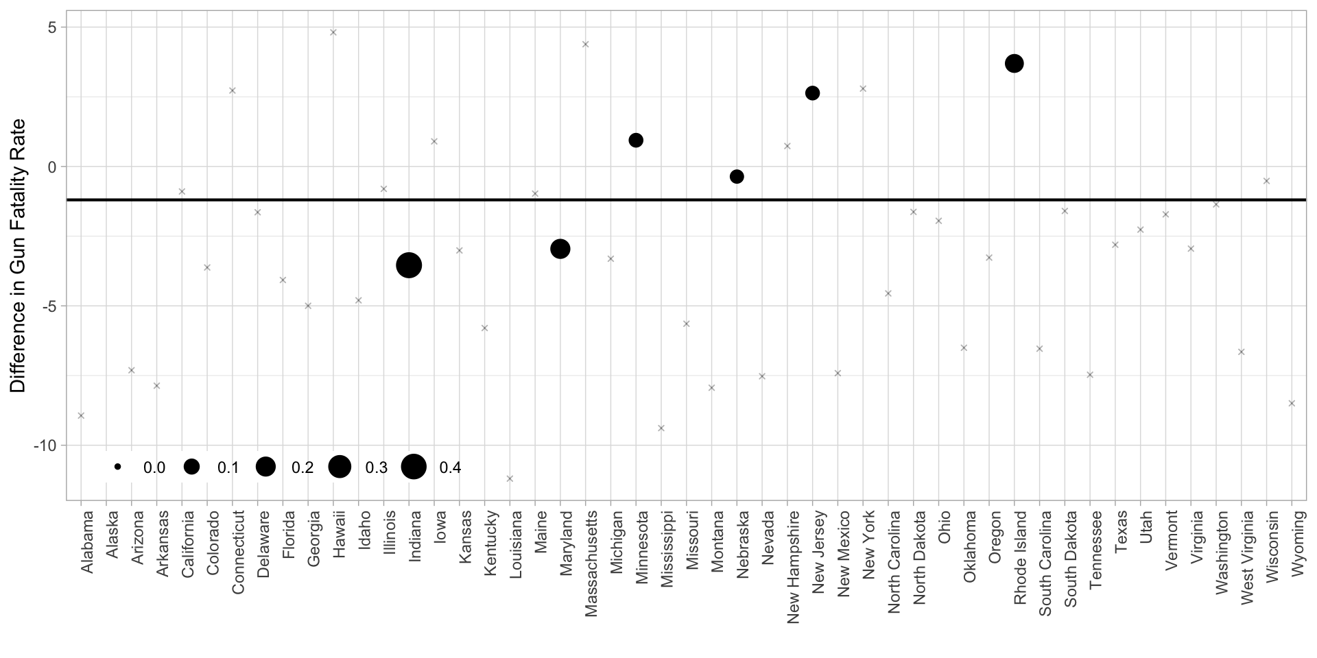
DID Estimates by State

• Constant weights: Each of the 49 control states receives weight 1/49 = 0.020408
• Adding Up: These weights all sum to 1
• Non-negativity: All of the weights are positive.
• Overall DID estimate is just a weighted average of these individual estimates.

Synthetic Control

Synthetic Control

1. No Intercept: \(\mu = 0\)

2. Adding Up: \(\sum_{i=1}^{n} \omega_i = 1\)

3. Non-negativity: \(\omega_i >= 0\) for all \(i\)

4. Constant weights: \(\omega_i = \bar \omega\) for all \(i\).

Synthetic Controls

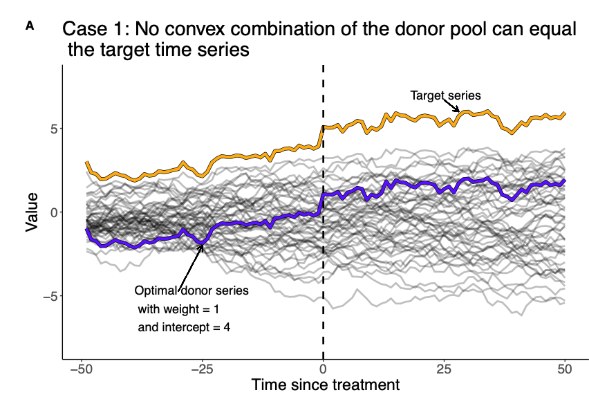
• Motivation: limit extrapolation bias that can occur when units with different pre-treatment characteristics are combined using a traditional adjustment, such as a linear regression (Kellogg et al. 2021).

Synthetic Control

• Imposing these constraints allows you to create a counterfactual whose outcome trajectory is within the support (“convex hull”) of donor units (i.e., other states)
• The counterfactual treated unit is simply a weighted sum of a subset of donors, with weights calculated to minimize the pre-intervention “distance” between the the treated unit and its synthetic counterfactual.
• Can use both lagged outcome and covariates to construct the weights.

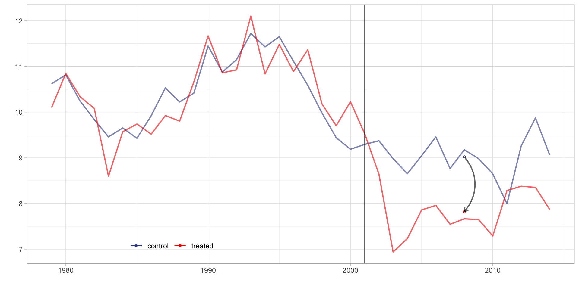
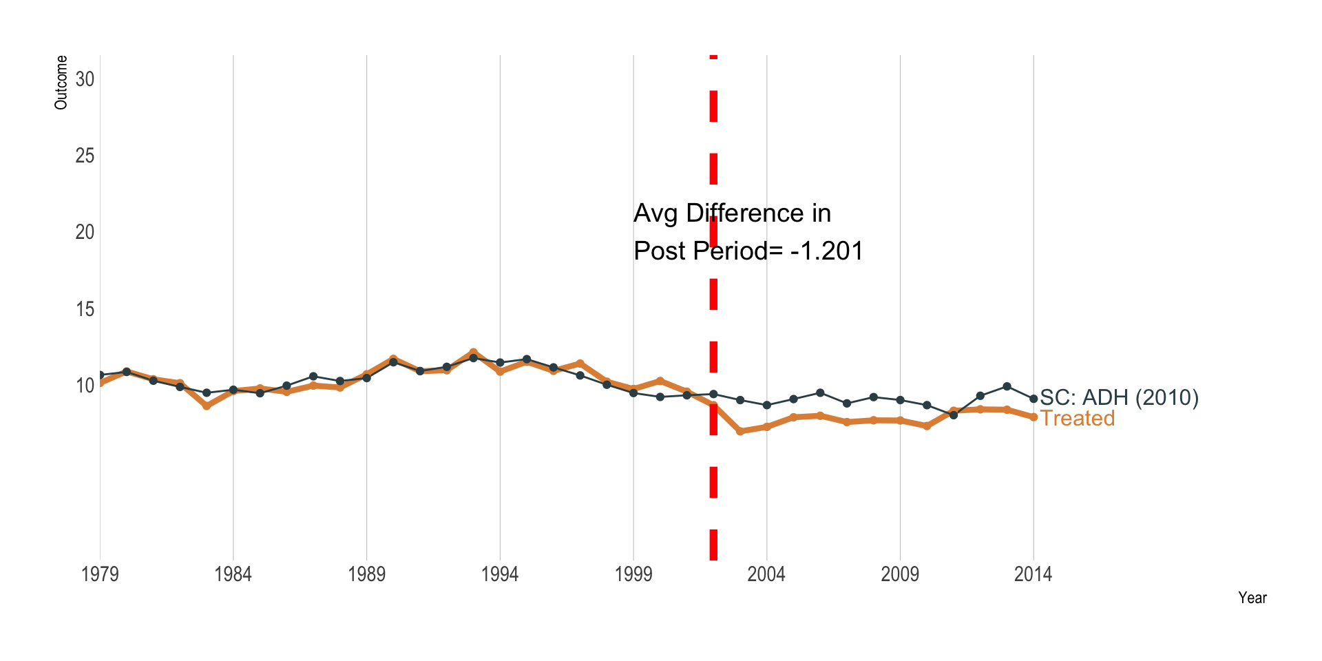
Synthetic Control Estimate

\(\hat \tau\) = -1.201

Weights: Synthetic Control

Synthetic Control From 100,000 feet

• At a high level, synthetic control methods choose a fixed set of weights that, when applied to the control units, produce a counterfactual to the treated unit.
• This counterfactual stands in as a “synthetic” treated unit that traces out what would have happened to the treatment unit had it never been treated.

Synthetic Control From Ground Level

• There are many approaches one could take to estimating the weights.
• We won’t get into all of them here, but many draw on innovative machine-learning methods.

Abadie, Diamond and Heinmueller (2010)

Match on pre-intervention outcome only:

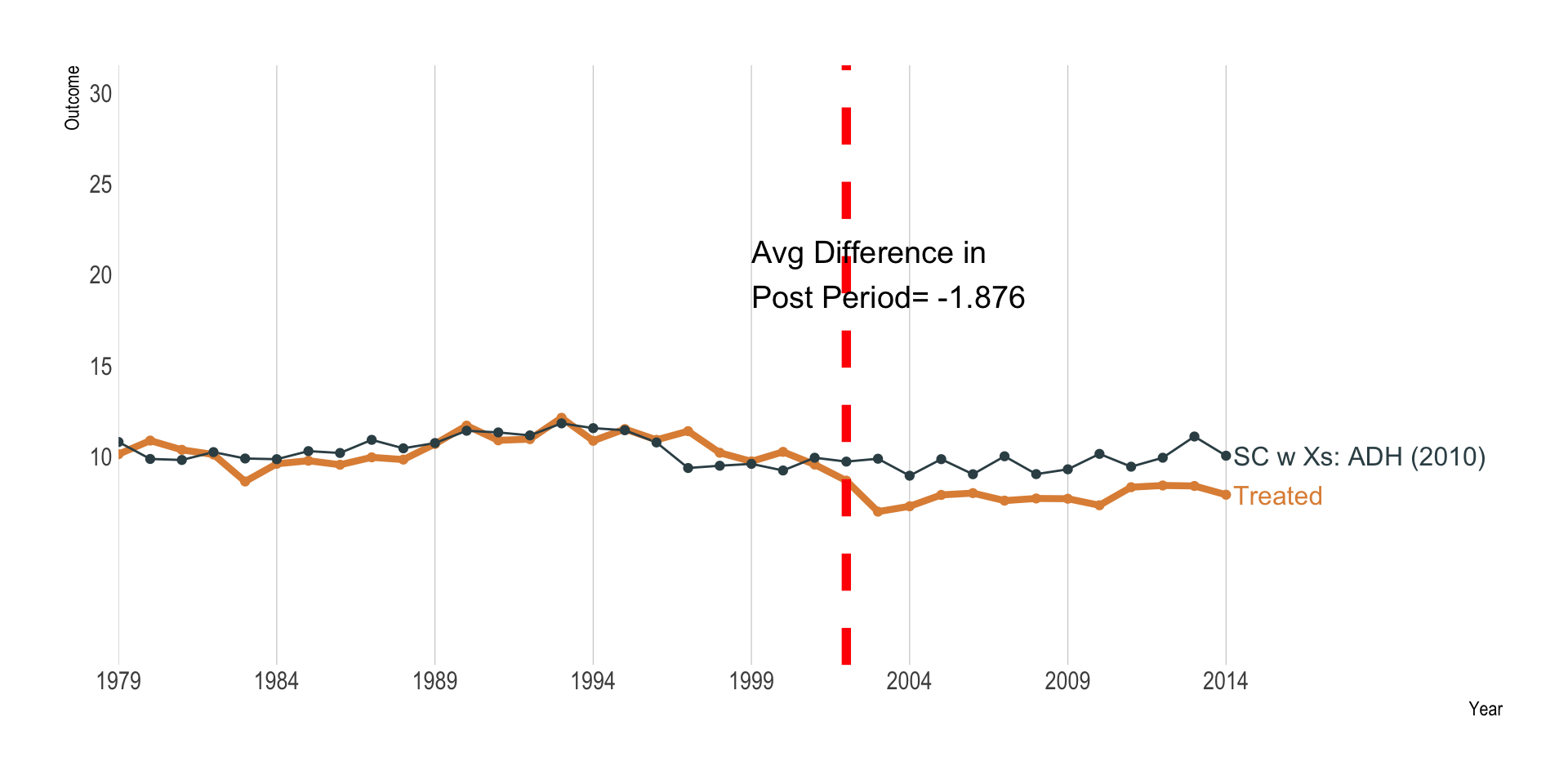
Abadie, Diamond and Heinmueller (2010)

Include state-level predictors:

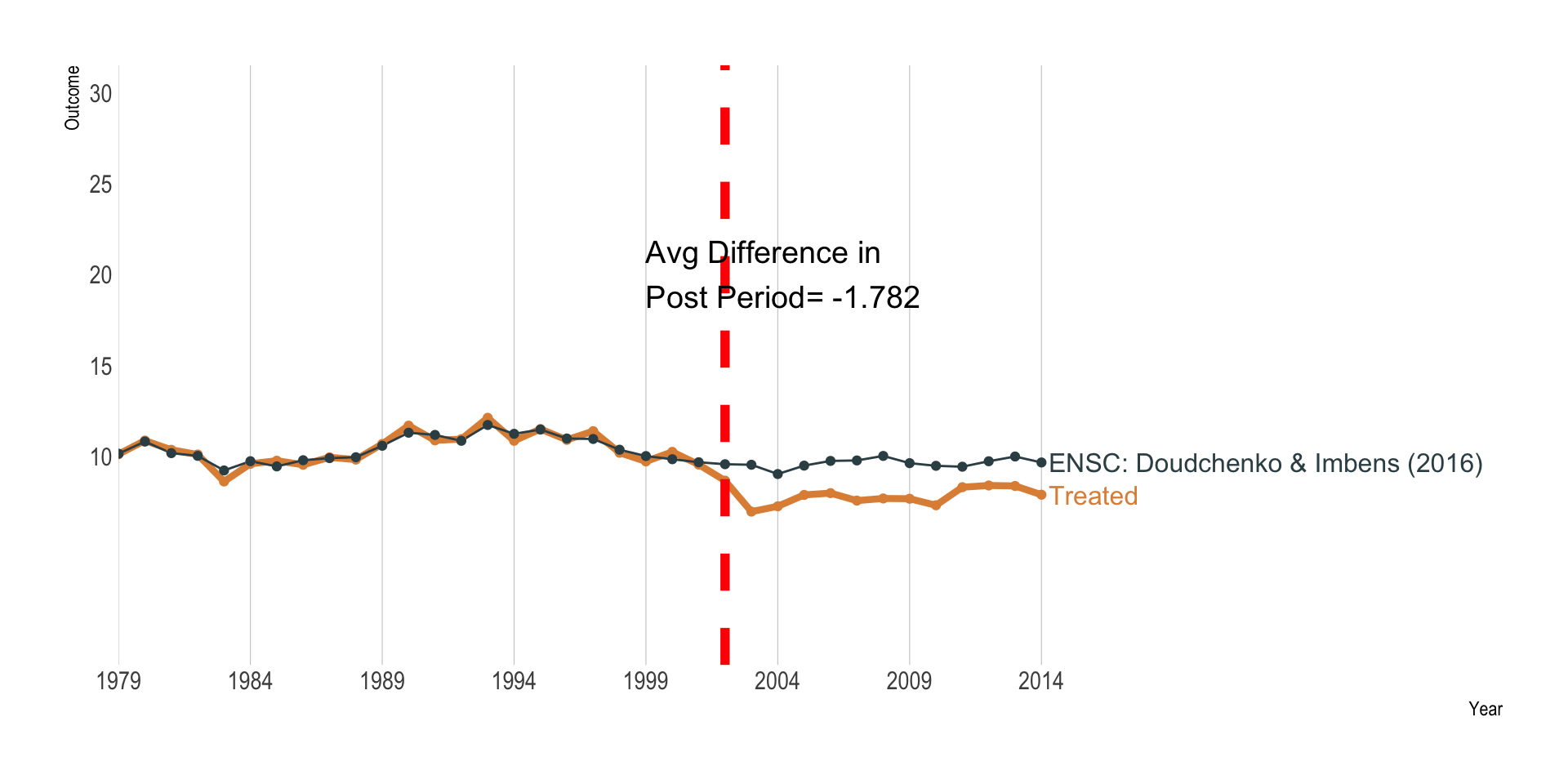
Elastic Net Synthetic Control

Doudchenko and Imbens (2017)

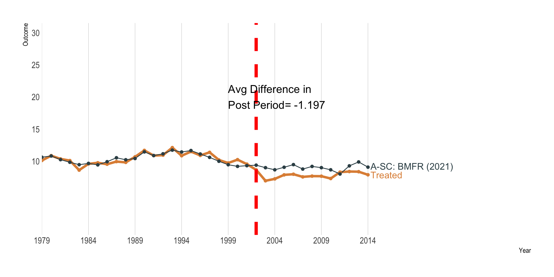
Augmented Synthetic Control

Ben-Michael, Feller and Rothstein (2021)

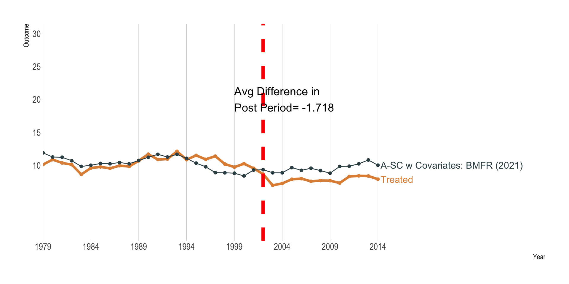
Augmented Synthetic Control

Using covariates to improve synthetic match

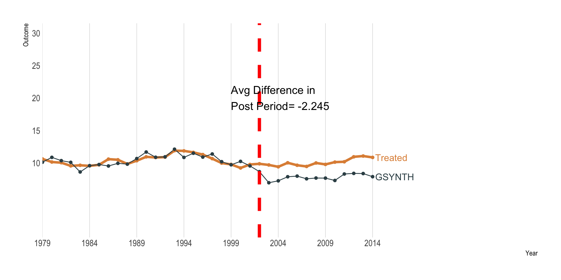
GSYNTH

• Generalized synthetic control method
• Imputes counterfactuals for each treated unit using control group information based on a linear interactive fixed effects model.
• Allows the treatment to be correlated with unobserved unit and time heterogeneity

GSYNTH

Inference

Inference for Synthetic Control

• Inference can be complex owing to the fact that often a single unit is “treated.”
  • Can’t appeal to large sample asymptotics.

Inference for Synthetic Control

• A standard approach: placebo treatments.
• Apply the synthetic control method to each donor unit, and collect the treatment effect estimates.
• Idea: the distribution of placebo effects give you a sense of what could happen under the null of no treatment effect.
• Can construct a p-value by asking where your estimate lies within this distribution.
• Analogous to randomization inference from last time.

Extensions of Synthetic Control

Synthetic Control with Staggered Adoption

• Xu (2017) (gsynth package)
• Ben-Michael, Feller, and Rothstein (2022) (augsynth package)

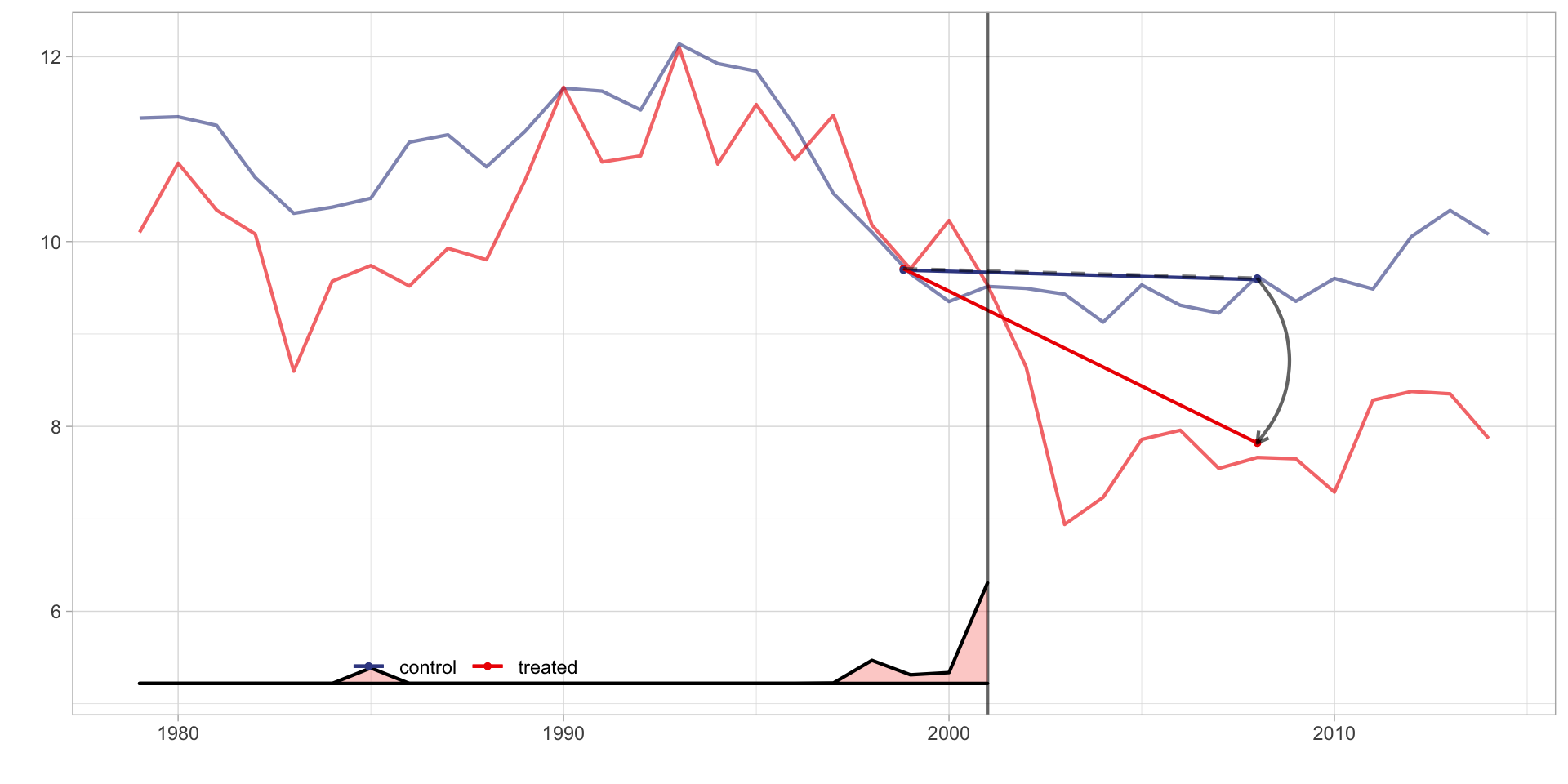
Synthetic Difference-in-Differences

• Arkhangelsky et al. (2019)
• Synthetic DID approach relaxes the parallel trends assumption.
• Key difference:
  1. Pre-intervention trends do not have to match exactly (i.e., 1. \(\mu = 0\) does not have to hold)
  2. Weighting is not equivalent across all time periods.

Synthetic Difference-in-Differences

\(\hat \tau\) = -1.783

Ensemble Methods