Nonlinear Difference-in-Differences
Motivation
- These slides will cover approaches for nonlinear difference-in-differences study designs.
- Types of outcomes covered:
- Binary outcomes
- Count (i.e., nonnegative) outcomes
- Categorical outcomes
What makes nonlinear DID different?
- DID analyses often rely on linear regression to estimate treatment effects.
- These analyses often rely on a linear, additive parallel trends assumption:
![]()
What makes nonlinear DID different?
- However, for binary and categorical outcomes (i.e., those taking multiple discrete values such as self-reported health status, health insurance type, etc.), the ordinal or multinomial regression models that are common in other settings are not well-suited to DID.
- Similarly, for count outcomes and those with “corner” solutions (i.e., outcomes that take a large number of zeros, such as medical spending), the usual (additive, linear) parallel trends assumption may not hold.
What makes nonlinear DID different?
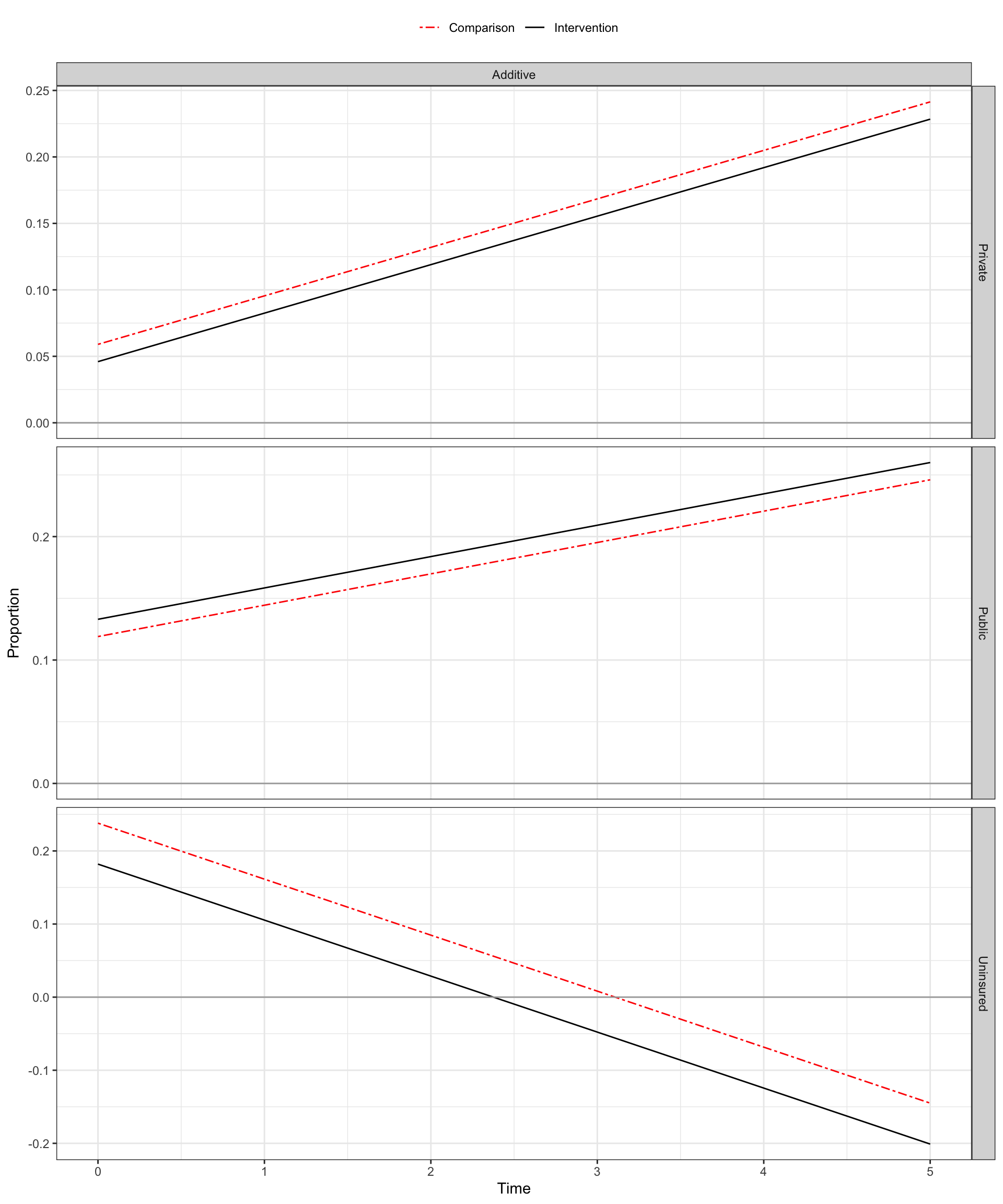
- Binary and count outcomes are bounded, so relying on an additive linear DID assumption of parallel trends can result in estimates that do not respect these bounds.
- Unless the two groups are already settled into an equilibrium (i.e., the proportions with each outcome value are constant over time) linear trends will yield outcome values with proportions below zero or above one.
What makes nonlinear DID different?
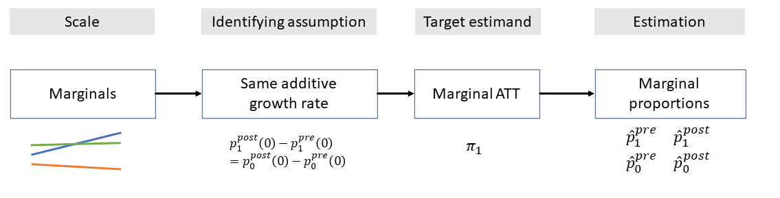
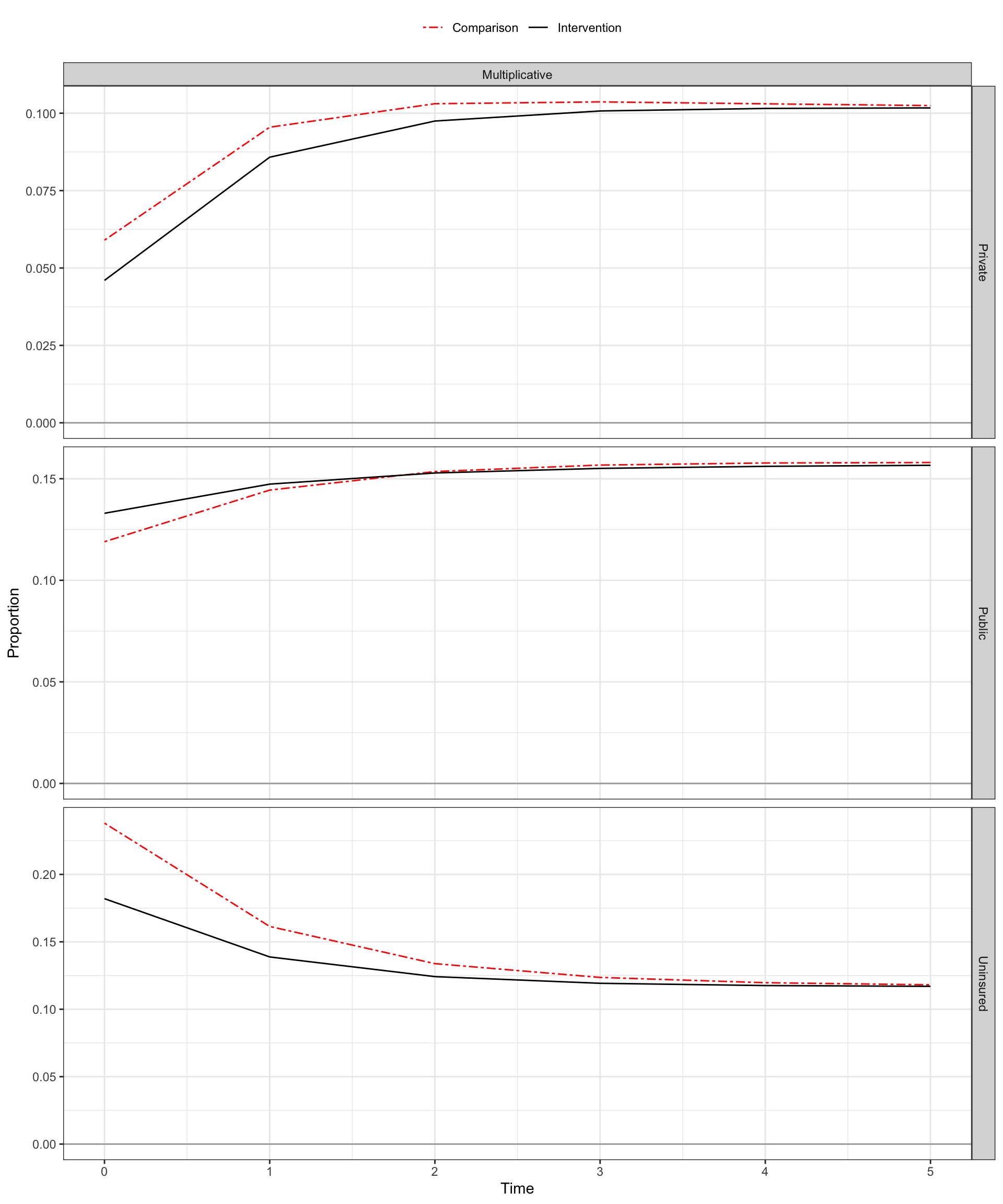
We want to rely on identifying assumptions that make sense given the scale of our outcome.
This means we need to be more flexible about the circumstances under which parallel trends holds:
- PT holds in the ratio of means (binary, count outcomes); see Wooldridge 2021
- PT holds in the transition dynamics (categorical outcomes); see Graves et al. 2022
- See related work by Athey and Imbens (2006) and Roth and Sant’Anna (2021)
What makes nonlinear DID different?
- For categorical outcomes, we may also be interested in transitions among outcome categories, not just overall changes in each category.
- Transitions among employment status (e.g., unemployed vs. employed vs. looking for work)
- Transitions in health insurance types (e.g., private vs. public vs. uninsured)
What makes nonlinear DID different?
For categorical outcomes, we may also be interested in transitions among outcome categories, not just overall changes in each category.
We could separately estimate DID for the marginal (i.e., overall) change in each category, and for separate outcomes defined for the various transition types.
However, this requires us to place parallel trends assumptions on two difference scales: the marginal scale and the transition scale.
- See Graves et al. (2022) for more.
Plan for Today
- Wooldridge (2021) “extended” DID framework as applied to nonlinear (binary, count) outcomes.
- Multinomial logit vs. transitions-based DID (Graves et al. 2022) for categorical outcomes.
Key Takeaways
- Extended DID framework can be used for nonlinear DID.
- It is still useful to compare linear DID to nonlinear estimates to see how sensitive estimates are to scale & functional form considerations.
Extended DID for Binary Outcomes
Binary Y, Common Treatment Timing
| Method | Estimation Formula |
|---|---|
| No Covariates | logit(y ~ I(w : d : f*) + factor(time) + d) |
| With Covariates | logit(y ~ I(w : d : f*) + I(w : d : f* : x_dm) + factor(time) + I(factor(time)*x) + d + x + I(d*x)) |
| Description | |
|---|---|
w |
Time-varying treatment indicator |
d |
Treatment cohort indicator |
f* |
Binary indicators for post-treatment times. |
factor(time) |
Time period fixed effects (dummies) |
x |
Covariate |
x_dm |
Demeaned covariate (x - mean(x|year>=tx_year)) |
Binary Y, Staggered Treatment Timing
| Method | Estimation Formula |
|---|---|
| No Covariates | logit(y ~ I(w : d* : f*) + factor(time) + d*) |
| With Covariates | logit(y ~ I( w : d* : f*) + I(w : d* : f* : x_dm_d*) + factor(time) + I(factor(time) : x) + d* + x + I(d* : x)) |
| Description | |
|---|---|
d* |
Treatment cohort indicators |
f* |
Binary indicators for post-treatment times. |
factor(time) |
Time period fixed effects (dummies) |
x |
Covariate |
x_dm_d* |
Demeaned covariate (x - mean(x|year>=tx_cohort_year)) |
Binary Outcome, Common Timing
Binary Y, Common Timing
- Note that in this example, treatment status is a function of the covariate
x. - Thus we need to condition on the covariate in order to identify the treatment effect.
Binary Y, Common Timing
- Get mean of
xfor the treatment cohort (i.e., observations whered=1) - Define a demeaned version of
xwhere we subtract that mean.
Binary Y, Common Timing
Logit regression:
Binary Y, Common Timing
| term | estimate |
|---|---|
| (Intercept) | -0.450 |
| I(w * d * f04) | 0.552 |
| I(w * d * f05) | 0.682 |
| I(w * d * f06) | 0.550 |
| I(w * d * f04 * x_dm) | -0.331 |
| I(w * d * f05 * x_dm) | -0.087 |
| I(w * d * f06 * x_dm) | 0.248 |
| f02 | 0.016 |
| f03 | -0.185 |
| f04 | 0.054 |
| f05 | -0.039 |
| f06 | 0.480 |
| I(f02 * x) | -0.075 |
| I(f03 * x) | 0.205 |
| I(f04 * x) | 0.294 |
| I(f05 * x) | 0.454 |
| I(f06 * x) | 0.156 |
| d | -2.186 |
| x | 0.505 |
| I(d * x) | 0.059 |
Binary Y, Common Timing
- Goal: Average Treatment Effect on the Treated (ATT) by post-treatment year.
- To caluclate, get marginal outcomes using prediction or the
marginscommand.
Binary Y, Common Timing
p04_w0 <-
  predict(fit_logit, type ="response",
    newdata = df %>% filter(d==1) %>% mutate(w=0,f02 =0, f03=0, f04=1, f05=0, f06=0))
p04_w1 <-
  predict(fit_logit, type ="response",
    newdata = df %>% filter(d==1) %>% mutate(w=1, f02 =0, f03=0, f04=1, f05=0, f06=0))

att04 <- mean(p04_w1)- mean(p04_w0)
att04
[1] 0.08866388library(marginaleffects)
marginaleffects(fit_logit,
newdata = datagrid(d=1,f02=0,f03=0,f04=1,f05=0,f06=0),
variables="w") %>%
select(term,dydx) term dydx
1 w 0.08045689Binary Y, Common Timing
| ATT | Truth | Logit Estimate | Linear Estimate |
|---|---|---|---|
| 2004 | 0.079 | 0.089 | 0.046 |
| 2005 | 0.118 | 0.122 | 0.026 |
| 2006 | 0.11 | 0.107 | -0.013 |
Count Y, Staggered Entry
Count Y, Staggered Entry
| Method | Estimation Formula |
|---|---|
| No Covariates | logit(y ~ I(w* : d* : f*) + factor(time) + d*) |
| With Covariates | logit(y ~ I(w* : d* : f*) + I(w : d* : f* : x_dm_d*) + factor(time) + I(factor(time) : x) + d* + x + I(d* : x)) |
| Description | |
|---|---|
w |
Time-varying treatment indicator |
d* |
Treatment cohort indicators |
f* |
Binary indicators for post-treatment times. |
factor(time) |
Time period fixed effects (dummies) |
x |
Covariate |
x_dm_d* |
Demeaned covariate (x - mean(x|year>=tx_cohort_year)) |
Count Y, Staggered Entry
Poisson regression (no covariates):
Count Y, Staggered Entry
Poisson regression (with covariates):
fit_poisson <-
    glm(y ~  I(w *  d4 * f04) + I(w *  d4 * f05) + I(w * d4* f06) +
             I(w *  d5 * f05) + I(w * d5* f06) +
             I(w *  d6 * f06) +
             I(w *  d4 * f04 * x_dm4) + I(w *  d4 * f05 * x_dm4) + I(w * d4* f06 * x_dm4) +
             I(w *  d5 * f05 * x_dm5) + I(w * d5* f06 * x_dm5) +
             I(w *  d6 * f06 * x_dm6) +
             f02 + f03 + f04 + f05 + f06 +
             I(f02 * x) + I(f03 * x) + I(f04 * x) + I(f05 * x) + I(f06 * x) +
             d4 + d5 + d6 +
             x +
             I(d4*x) + I(d5*x) + I(d6*x),
      family = 'poisson',
data = df)"| term | no_x | with_x |
|---|---|---|
| (Intercept) | 1.639 | 1.174 |
| I(w * d4 * f04) | 0.877 | 0.858 |
| I(w * d4 * f05) | 0.494 | 0.481 |
| I(w * d4 * f06) | 1.004 | 1.007 |
| I(w * d5 * f05) | 1.255 | 1.237 |
| I(w * d5 * f06) | 1.132 | 1.095 |
| I(w * d6 * f06) | 1.171 | 1.089 |
| f02 | 0.341 | 0.604 |
| f03 | 0.415 | 0.818 |
| f04 | 0.571 | 0.778 |
| f05 | 0.523 | 0.726 |
| f06 | 0.532 | 0.811 |
| d4 | -0.907 | -0.492 |
| d5 | -1.067 | -0.92 |
| d6 | -1.12 | -0.879 |
| I(w * d4 * f04 * x_dm4) | 0.604 | |
| I(w * d4 * f05 * x_dm4) | -0.226 | |
| I(w * d4 * f06 * x_dm4) | -0.019 | |
| I(w * d5 * f05 * x_dm5) | 0.28 | |
| I(w * d5 * f06 * x_dm5) | 0.688 | |
| I(w * d6 * f06 * x_dm6) | 1.01 | |
| I(f02 * x) | -0.268 | |
| I(f03 * x) | -0.416 | |
| I(f04 * x) | -0.208 | |
| I(f05 * x) | -0.205 | |
| I(f06 * x) | -0.286 | |
| x | 0.492 | |
| I(d4 * x) | -0.43 | |
| I(d5 * x) | -0.176 | |
| I(d6 * x) | -0.264 |
Count Y, Staggered Entry
- Goal: Average Treatment Effect on the Treated (ATT) by cohort and post-treatment year.
- To caluclate, get marginal outcomes using prediction or the
marginscommand.
d04_f04_w0 <- predict(fit_poisson, type ="response",
                    newdata = df_st %>% filter(d4==1) %>%
                    mutate(w=0,d4=1, d5=0, d6=0, f02 =0, f03=0, f04=1, f05=0, f06=0))

d04_f04_w1 <- predict(fit_poisson, type ="response",
                    newdata = df_st %>% filter(d4==1) %>%
                    mutate(w=1, d4=1, d5=0, d6=0, f02 =0, f03=0, f04=1, f05=0, f06=0))

att04 <- mean(d04_f04_w1)- mean(d04_f04_w0)
att04
[1] 5.166275Count Y, Staggered Entry
| Cohort | Year | Truth | Poisson No X | Poisson w X | Linear w X |
|---|---|---|---|---|---|
| 2004 | 2004 | 5.588 | 5.166 | 5.153 | 4.202 |
| 2004 | 2005 | 2.473 | 2.242 | 2.227 | 1.235 |
| 2004 | 2006 | 4.722 | 6.121 | 6.133 | 5.064 |
| 2005 | 2005 | 3.638 | 7.494 | 7.478 | 6.638 |
| 2005 | 2006 | 5.16 | 6.339 | 6.362 | 5.441 |
| 2006 | 2006 | 3.439 | 6.367 | 6.416 | 5.652 |
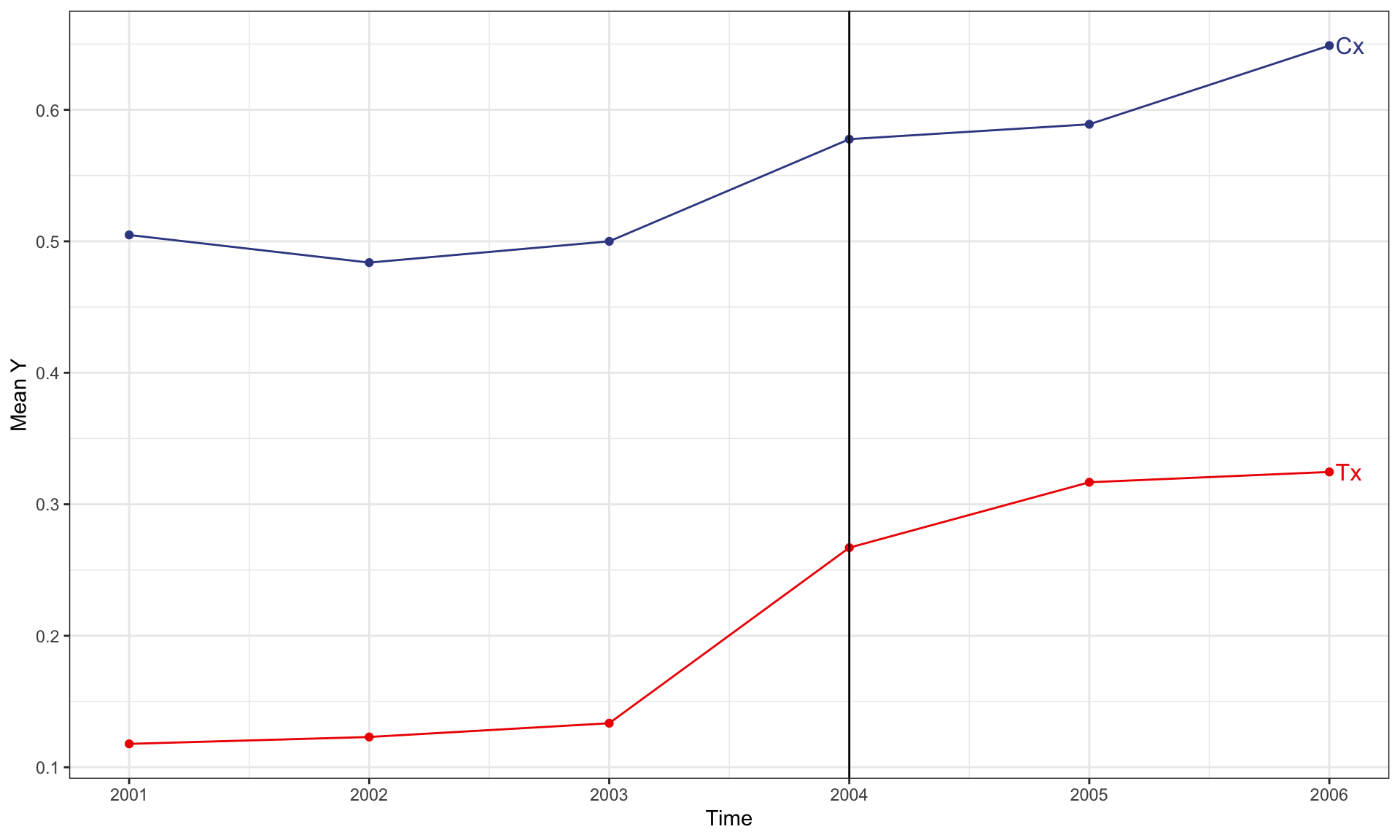
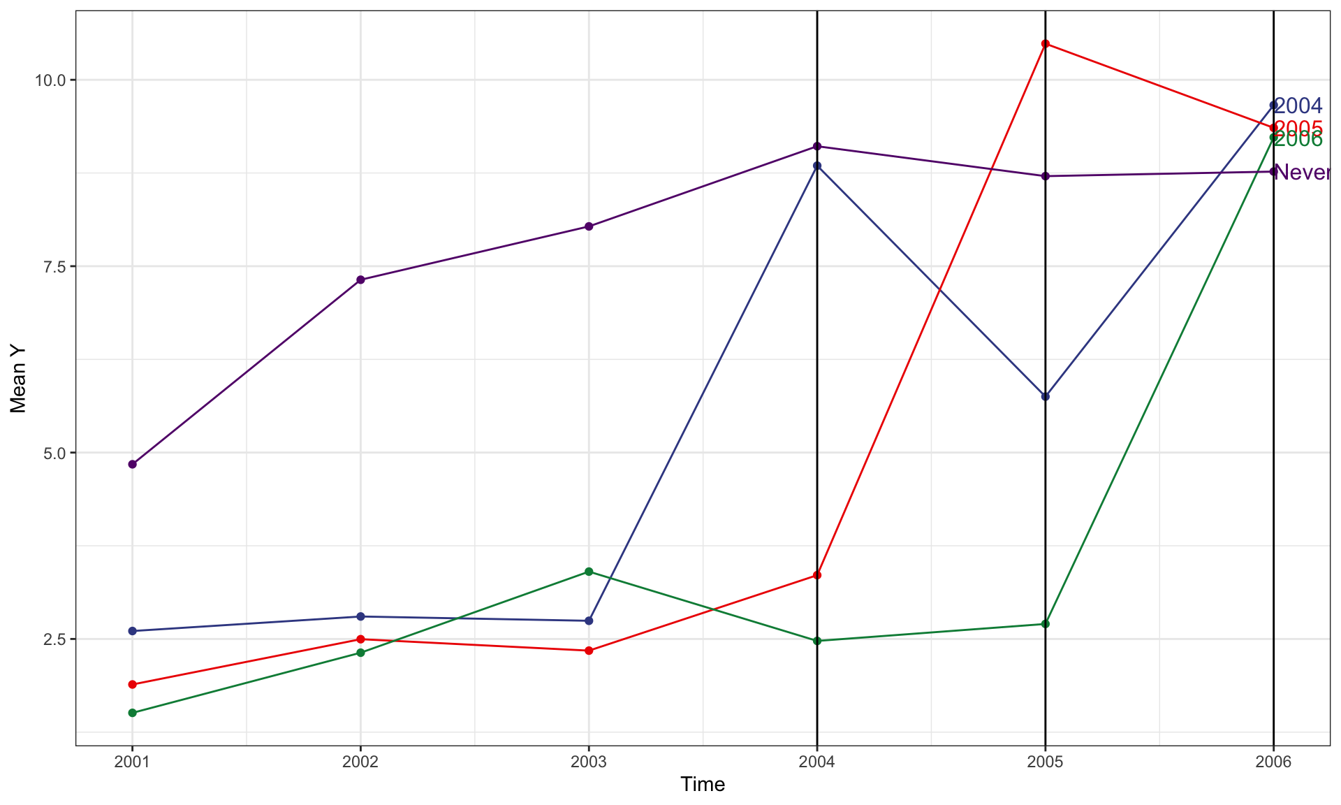
How Well Do the Estimators Perform?
ATTs are time varying but do not vary with X:
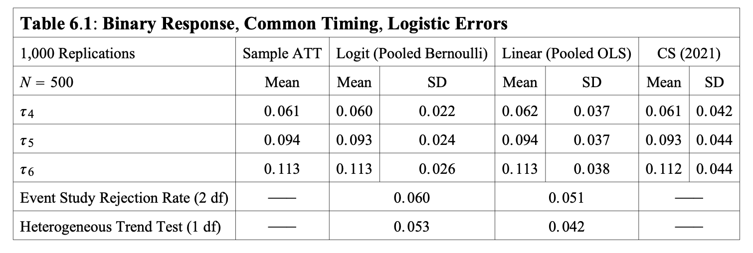
Source: Wooldridge (2022) ‘Simple Approaches to Nonlinear Difference-in-Differences with Panel Data’
How Well Do the Estimators Perform?
ATTs time varying and increasing:
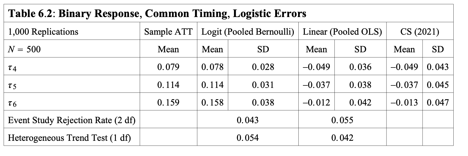
Source: Wooldridge (2022) ‘Simple Approaches to Nonlinear Difference-in-Differences with Panel Data’
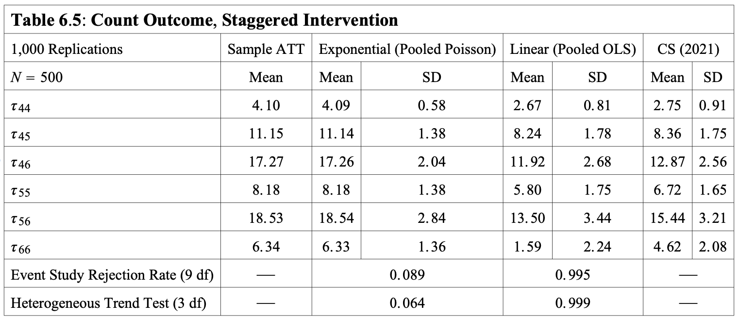
How Well Do the Estimators Perform?
Count outcome with mass at 0:
Extended Nonlinear DID: Concluding Remarks
- Extended DID applies well for nonlinear settings.
- You can obtain a full set of ATTs indexed by cohort/calendar time.
- Alternatively, you can aggregate into some other quantity of interest (e.g., overall effect, relative time effects, etc.)
Extended Nonlinear DID: Concluding Remarks
Can use either an imputation approach (i.e., fit the nonlinear model on only comparison observations, then impute predicted missing potential outcomes for treated)
Often easier to use pooled estimation (as we did here) for conducting inference (e.g., standard errors)
Extended Nonlinear DID: Concluding Remarks
Nonlinear models have essentially no bias when the conditional mean is correctly specified.
- They also work reasonably well under some misspecifications.
Easy to apply methods to settings where all units are eventually treated.
Method can also handle staggered exit by including a richer set of cohort dummy variables.
Extended Nonlinear DID: Concluding Remarks
Can also accomodate multiple (i.e., non-binary treatments) by replacing
wwith treatment-level indicators.Methods should extend to repeated cross sections, but details are still pending.
End for today!
Categorical Outcomes
| Marginal Effect Model Coefficients (std. error) Based on Linear Probability Model | ||||
| ESI | NG | PUB | UNIN | |
|---|---|---|---|---|
| Intercept | 0.3134 (0.0055) | 0.079 (0.0031) | 0.4561 (0.0059) | 0.1515 (0.0041) |
| post | -0.0032 (0.0058) | -0.001 (0.0033) | 0.0094 (0.0063) | -0.0052 (0.0044) |
| post.z | -0.0164 (0.0083) | -0.007 (0.0047) | 0.051 (0.0089) | -0.0276 (0.0062) |
| X | -0.0033 (0.0071) | 0.001 (0.0041) | 7e-04 (0.0077) | 0.0017 (0.0053) |
| z | 0.0057 (0.0058) | -0.0052 (0.0033) | 0.0075 (0.0063) | -0.0081 (0.0044) |
Categorical Outcomes
# weights:  24 (15 variable)
initial  value 69314.718056
iter  10 value 61818.934305
iter  20 value 59087.519803
final  value 59077.301898
converged| Marginal Effect Model Coefficients Based on Multinomial Logit Model | |||
| NG | PUB | UNIN | |
|---|---|---|---|
| Intercept | -1.3791 (0.0476) | 0.3752 (0.0274) | -0.7278 (0.0376) |
| post | -0.0018 (0.0504) | 0.0306 (0.0294) | -0.0244 (0.0398) |
| post.z | -0.0473 (0.0731) | 0.1553 (0.0413) | -0.17 (0.0581) |
| X | 0.0237 (0.063) | 0.0122 (0.0357) | 0.0229 (0.05) |
| z | -0.086 (0.0509) | -0.0019 (0.0293) | -0.0726 (0.0399) |
Categorical Outcomes
| Marginal Effect Estimates Based on Recycled Predictions from a Multinomial Logit Model | |||||
| DID Estimate | Comparison Group | Intevention Group | |||
|---|---|---|---|---|---|
| ATT | Pre-Intervention | Post-Intervention | Pre-Intervention | Post-Intervention | |
| ESI | −0.0164 | 0.312 | 0.309 | 0.318 | 0.298 |
| NG | −0.00696 | 0.0794 | 0.0785 | 0.0742 | 0.0663 |
| PUB | 0.0510 | 0.456 | 0.466 | 0.464 | 0.524 |
| UNIN | −0.0276 | 0.152 | 0.147 | 0.144 | 0.111 |
Categorical Outcomes
| Summary of Marginal Effect Point Estimates Using Nonparametric Transitions Estimator | ||||||
| ATT | p | R_DD | ||||
|---|---|---|---|---|---|---|
| ESI | NG | PUB | UNIN | |||
| ESI | −0.0126 | 0.318 | −0.0155 | −0.0110 | 0.0364 | −0.00992 |
| NG | −0.0102 | 0.0742 | −0.0606 | −0.0487 | 0.130 | −0.0210 |
| PUB | 0.0544 | 0.464 | −0.00160 | −0.00421 | 0.0118 | −0.00599 |
| UNIN | −0.0317 | 0.144 | −0.0168 | −0.00804 | 0.192 | −0.168 |
Categorical Outcomes
| Linear Transition Regression Model Coefficients (SE) | |||
| Outcome | |||
|---|---|---|---|
| ESI | NG | PUB | |
| ESI | 0.596 (0.008) | 0.062 (0.005) | 0.253 (0.009) |
| ESI.z | -0.015 (0.009) | -0.011 (0.006) | 0.036 (0.01) |
| NG | 0.297 (0.014) | 0.335 (0.008) | 0.237 (0.015) |
| NG.z | -0.061 (0.019) | -0.049 (0.011) | 0.13 (0.02) |
| PUB | 0.155 (0.007) | 0.036 (0.004) | 0.749 (0.008) |
| PUB.z | -0.002 (0.008) | -0.004 (0.005) | 0.012 (0.008) |
| UNIN | 0.137 (0.011) | 0.104 (0.006) | 0.225 (0.011) |
| UNIN.z | -0.017 (0.014) | -0.008 (0.008) | 0.192 (0.015) |
| X | 0.015 (0.009) | 0.001 (0.005) | -0.016 (0.01) |
Categorical Outcomes
| Summary of Marginal Effect Point Estimates Using Regression-Based Transitions Estimator | ||||||
| ATT | p | R_DD | ||||
|---|---|---|---|---|---|---|
| ESI | NG | PUB | UNIN | |||
| ESI | −0.0125 | 0.318 | −0.0154 | −0.0110 | 0.0363 | −0.00992 |
| NG | −0.0102 | 0.0742 | −0.0606 | −0.0487 | 0.130 | −0.0210 |
| PUB | 0.0544 | 0.464 | −0.00155 | −0.00420 | 0.0117 | −0.00599 |
| UNIN | −0.0317 | 0.144 | −0.0168 | −0.00804 | 0.192 | −0.168 |
Categorical Outcomes
# weights:  40 (27 variable)
initial  value 34657.359028
iter  10 value 25809.195153
iter  20 value 24695.991682
iter  30 value 24245.070325
final  value 24204.028126
converged| Tansition Model Coefficients (std. error) Based on Multinomial Logit Model | |||
| NG | PUB | UNIN | |
|---|---|---|---|
| ESI | -2.2432 (0.0822) | -0.8497 (0.0476) | -1.8871 (0.0702) |
| ESI.z | -0.1668 (0.0991) | 0.1636 (0.0529) | -0.0933 (0.0834) |
| NG | 0.1201 (0.0918) | -0.2306 (0.0919) | -0.8111 (0.1119) |
| NG.z | 0.0653 (0.1204) | 0.672 (0.123) | 0.0476 (0.1588) |
| PUB | -1.4798 (0.0906) | 1.5709 (0.0463) | -0.9485 (0.0748) |
| PUB.z | -0.114 (0.1114) | 0.0254 (0.0512) | -0.0939 (0.0904) |
| UNIN | -0.3089 (0.1046) | 0.4554 (0.0828) | 1.3372 (0.079) |
| UNIN.z | 0.0429 (0.1371) | 0.7582 (0.1083) | -0.2531 (0.1022) |
| X | -0.0458 (0.0942) | -0.1038 (0.0565) | -0.0652 (0.0798) |
Categorical Outcomes
| Summary of Marginal Effect Point Estimates Using Multinomial Regression-Based Transitions Estimator | ||||||
| ATT | p | R_DD | ||||
|---|---|---|---|---|---|---|
| ESI | NG | PUB | UNIN | |||
| ESI | −0.0127 | 0.318 | −0.0158 | −0.0111 | 0.0371 | −0.0102 |
| NG | −0.0104 | 0.0742 | −0.0604 | −0.0501 | 0.132 | −0.0217 |
| PUB | 0.0551 | 0.464 | −0.00154 | −0.00413 | 0.0116 | −0.00594 |
| UNIN | −0.0320 | 0.144 | −0.0168 | −0.00838 | 0.195 | −0.169 |