Extending Difference-in-Differences
Outline
- Review DID identifying assumptions.
- DID Estimators
- Canonical \(2\times2\)
- Two-Way Fixed Effects (TWFE) DID
- TWFE Event Study DID
- Extended DID (TWFE, random effects, and pooled OLS)
Notation
- Binary treatment
- \(y_z^{t}(d)\) is the potential outcome in treatment group \(z\) (e.g., comparison, intervention) at time \(t\).
- \(y_1^{post}(1)\) is the observed post-intervention outcome of individuals in the intervention group.
- \(y_1^{post}(0)\) is the counterfactual post-intervention outcome of individuals in the intervention group.
Estimand of Interest
- Average effect of treatment on the treated (ATT)
\[
\pi_1 = y_1^{post}(1) - y_1^{post}(0)
\]
- This is the difference in the post-period potential outcome under treatment versus no treatment in the intervention group.
Estimand of Interest
- In the post-period, we only observe the intervention group under treatment, so its potential outcome distribution under no treatment, \(y_1^{post} (0)\), is an unobservable counterfactual.
- Thus, we must make identifying assumptions to estimate \(\pi_1\) with observable quantities.
Identifying Assumptions
- We can use a parallel trends assumption that the comparison group’s (additive, linear) pre- to post-period change in untreated potential outcome distribution is the same as the intervention group’s:
\[
y_0^{post} (0)-y_0^{pre}(0)=y_1^{post} (0)-y_1^{pre} (0)
\]
Identifying Assumptions
- Solving for the unobservable quantity we need
\[
y_1^{post} (0)=y_0^{post} (0)-y_0^{pre} (0)+y_1^{pre} (0)
\]
Identifying Assumptions
- Plugging in to the target estimand, we have
\[
\pi_1=y_1^{post} (1)-y_0^{post} (0)+y_0^{pre} (0)-y_1^{pre} (0).
\]
Estimator
- We further assume that observed outcomes correspond to potential outcomes under observed treatments (called the consistency assumption) and write the estimand in terms of observable quantities,
\[
\pi_1=(y_1^{post}-y_1^{pre} )-(y_0^{post}-y_0^{pre} )
\] where \(y_z^{t}\) is the observed outcome in group \(z\) during period \(t\).
Estimator
- For the canonical 2x2 case, we can estimate this quantity using simple summaries of the proportions in each outcome value, group, and period.
- Alternatively, if we need to condition on covariates to make identifying assumptions plausible, we can use regression or semi-parametric approaches.
Dimensions of an Intervention and its Effect
- Number of treatment groups (single, multiple).
- Treatment timing (single, staggered rollout).
- Cohort-level treatment effect heterogeneity (yes, no)
- Treatment effect type (constant, dynamic)
DID Estimators
Common Treatment Time, Constant Treatment Effects
| tx_groups |
timing |
het |
tx_effect |
| Single |
Single |
No |
Constant |
![]()
DID Estimators
Common Treatment Time, Dynamic Treatment Effects
| tx_groups |
timing |
het |
tx_effect |
| Single |
Single |
No |
Dynamic |
![]()
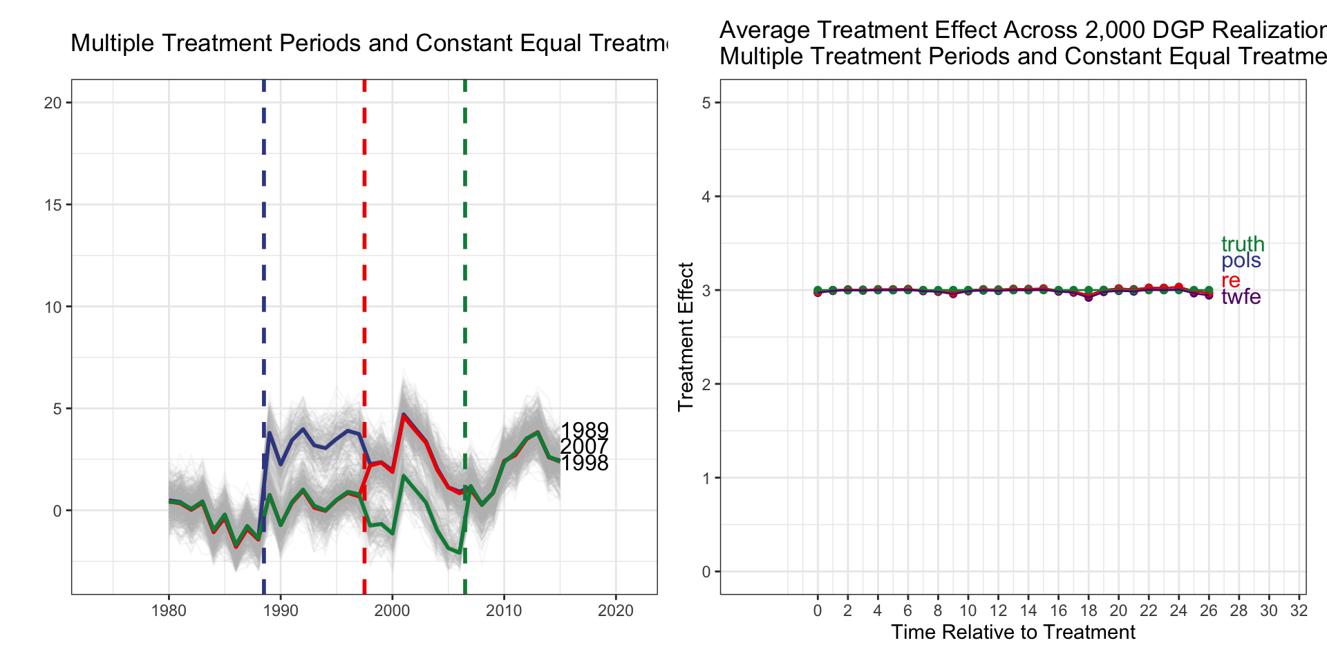
DID Estimators
Multiple Treatment Periods and Constant Equal Treatment Effects
| tx_groups |
timing |
het |
tx_effect |
| Multiple |
Staggered |
No |
Constant |
![]()
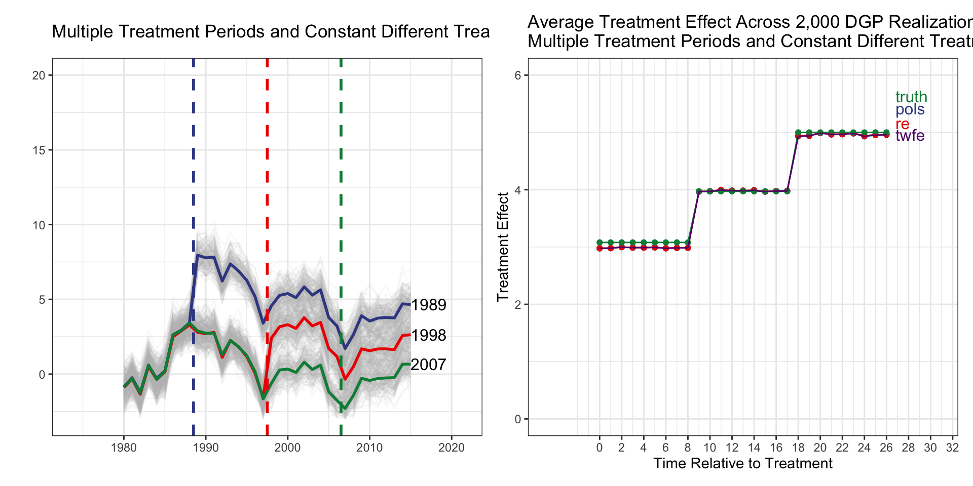
DID Estimators
Multiple Treatment Periods and Constant Different Treatment Effects, All Groups Eventually Treated
| tx_groups |
timing |
het |
tx_effect |
| Multiple |
Staggered |
Yes |
Constant |
![]()
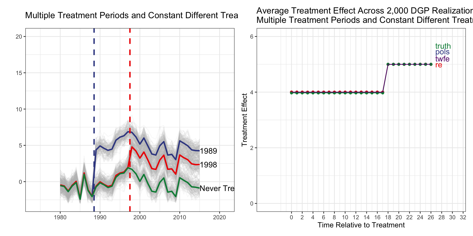
DID Estimators
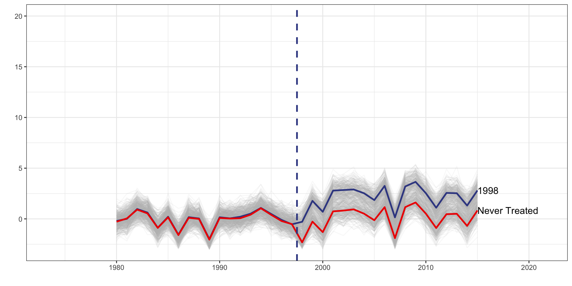
Multiple Treatment Periods and Constant Different Treatment Effects, Never Treated Group
| tx_groups |
timing |
het |
tx_effect |
| Multiple |
Staggered |
Yes |
Constant |
![]()
DID Estimators
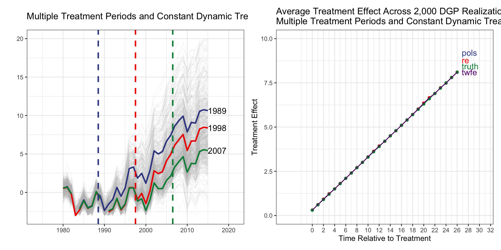
Multiple Treatment Periods and Constant Dynamic Treatment Effects
| tx_groups |
timing |
het |
tx_effect |
| Multiple |
Staggered |
No |
Dynamic |
![]()
DID Estimators
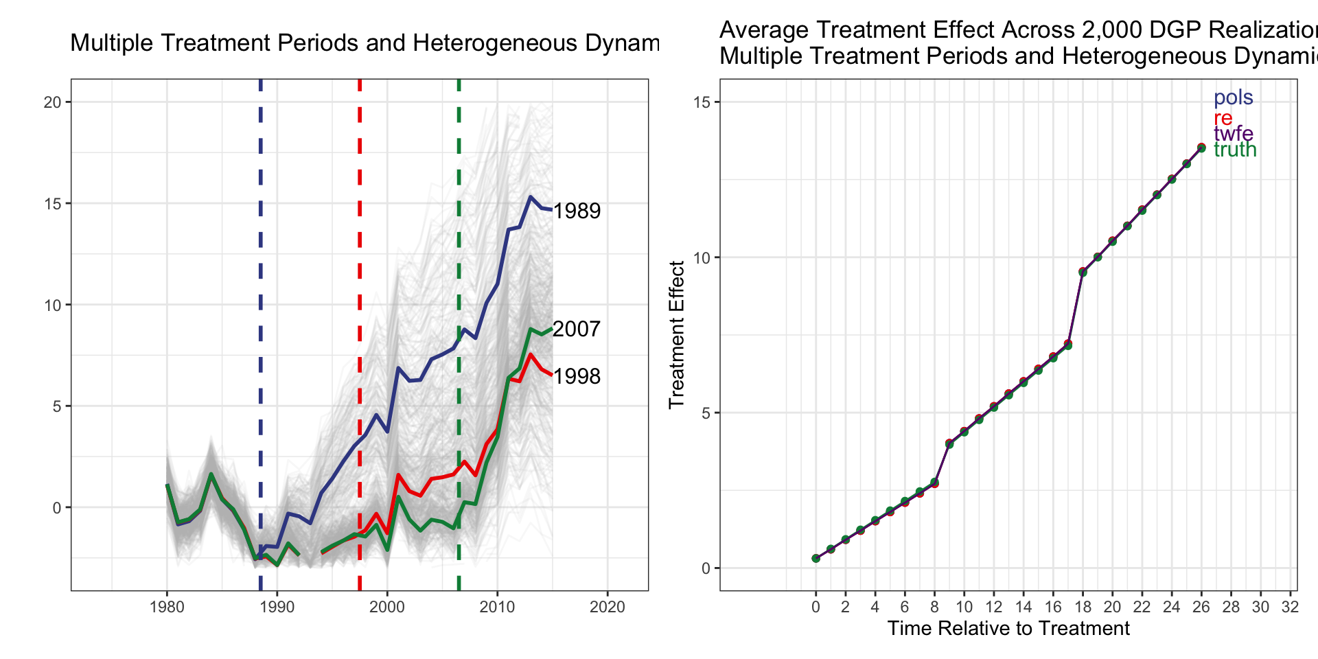
Multiple Treatment Periods and Heterogeneous Dynamic Treatment Effects
| tx_groups |
timing |
het |
tx_effect |
| Multiple |
Staggered |
Yes |
Dynamic |
![]()
DID Estimators
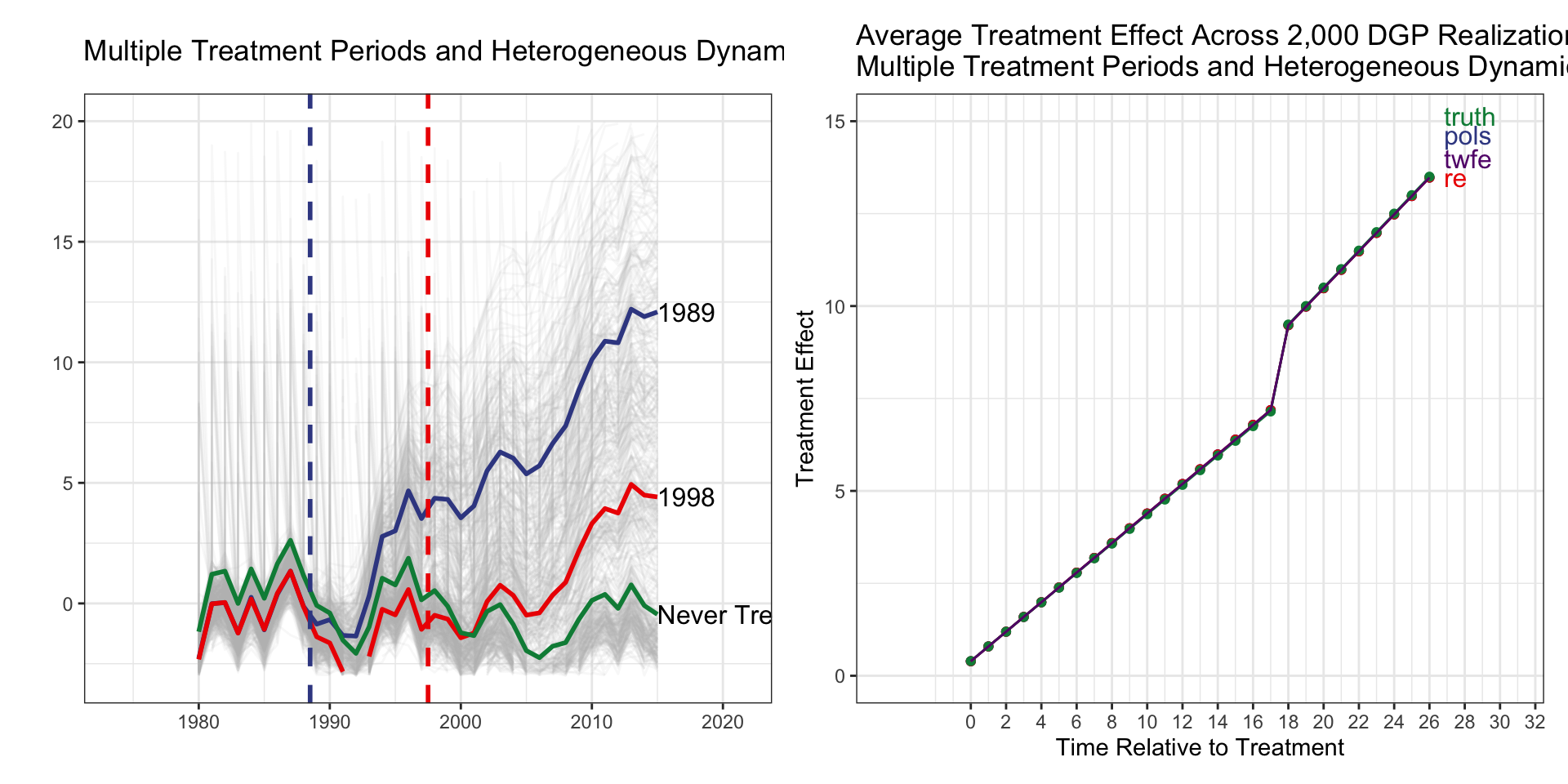
Multiple Treatment Periods and Heterogeneous Dynamic Treatment Effects, Never Treated Group
| tx_groups |
timing |
het |
tx_effect |
| Multiple |
Staggered |
Yes |
Dynamic |
![]()
DID Estimators
- Two-Way Fixed Effects DID (“TWFE”)
- Two-Way Fixed Effects Event Study DID (“TWFE-ES”)
- Extended Differences-in-Differences (“E-DID”)
- Extended Two-Way Fixed Effect DID (“E-TWFE”)
- Extended Pooled OLS (“E-POLS”)
- Extended Random Effect (“Extended Two Way Mundlak” or “E-TWM”)
Two-Way Fixed Effects DID Estimator
- A common approach is a so-called “two-way fixed effects” difference-in-differences estimator:
\[
y_{it} = \tau D_{it} + \delta_i + \gamma_t + \epsilon_{it}
\]
Two-Way Fixed Effects DID Estimator
\[
Y_{it} = \tau D_{it} + \delta_i + \gamma_t + \epsilon_{it}
\]
\(D_{it}\) is a binary treatment indicator set to 1 if the individual is in the treated group and the the observation is in the post-treatment period.
\(\delta_i\) and \(\gamma_t\) are unit and time fixed effects, respectively.
Inclusion of unit and time fixed effects flexibly accounts for both unit-specific (but time-invariant) and time-specific (but unit-invariant) unobserved confounders.
Two-Way Fixed Effects DID Estimator
\[
Y_{it} = \tau D_{it} + \delta_i + \gamma_t + \epsilon_{it}
\]
Can think of \(\delta_i = h(\mathbf{U_i})\) and \(\gamma_t = f(\mathbf{V_t})\), where \(\mathbf{U_i}\) are unit specific confounders and \(\mathbf{V_t}\) are time-specific confounders that are common causes of the treatment and the outcome.
\(h(.)\) and \(f(.)\) are arbitrary functions that we do not necessarily know the structure of.
Two-Way Fixed Effects DID Estimator
\[
Y_{it} = \tau D_{it} + \delta_i + \gamma_t + \epsilon_{it}
\]
While the model is assuming there are no interactions between confounders \(\mathbf{U_i}\) and \(\mathbf{V_t}\), there are no functional form restrictions placed on \(h(.)\) and \(f(.)\).
So the model is only making assumptions on the additivity and separability of unobserved confounders.
Source: Imai and Kim
Two-Way Fixed Effects DID Estimator
| Single |
Single |
No |
Constant |
Yes |
| Single |
Single |
No |
Dynamic |
Yes1 |
| Multiple |
Single |
No |
Constant |
Yes |
| Multiple |
Single |
Yes |
Constant |
No |
| Multiple |
Staggered |
No |
Constant |
No |
| Multiple |
Staggered |
Yes |
Constant |
No |
| Multiple |
Single |
No |
Dynamic |
No |
| Multiple |
Single |
Yes |
Dynamic |
No |
| Multiple |
Staggered |
No |
Dynamic |
No |
| Multiple |
Staggered |
Yes |
Dynamic |
No |
TWFE Event Study DID Estimator
- Another option is to fit a two-way fixed effects event study DID model.
TWFE Event Study DID Estimator
\(Y_{it} = \delta_i + \gamma_t + \gamma_k^{-K}D_{it}^{<-K} + \sum_{k=-K}^{-2}\gamma_k^{lead}D_{it}^k+\sum_{k=0}^{L}\gamma_k^{lag}D_{it}^k + \gamma_k^{L+}D_{it}^{>L} + \epsilon_{it}\)
\(\delta_i\) and \(\gamma_t\) are unit and time fixed effects, respectively.
We use \(K\) lags and \(L\) leads, and \(D_{i,t}^k\) are event study dummy variables that take a value of one if unit \(i\) is \(k\) periods away from initial treatment time at time \(t\) and zero otherwise.
TWFE Event Study DID Estimator
We may not want to specify every lead and lag available in our data. As such, \(D_{it}^{<-K}\) and \(D_{it}^{>L}\) are Pre and Post variables if the observation is more than \(K\) time periods away in the pre period, and more than \(L\) periods away in the post period.
Also note that the indicator for the time period just before policy adoption, i.e., \(D_{it}^{-1}\) is the excluded category.
TWFE Event Study DID Estimator
| Single |
Single |
No |
Constant |
Yes |
Yes |
| Single |
Single |
No |
Dynamic |
Yes1 |
Yes |
| Multiple |
Single |
No |
Constant |
Yes |
Yes |
| Multiple |
Single |
Yes |
Constant |
No |
No |
| Multiple |
Staggered |
No |
Constant |
No |
Yes |
| Multiple |
Staggered |
Yes |
Constant |
No |
No |
| Multiple |
Single |
No |
Dynamic |
No |
No |
| Multiple |
Single |
Yes |
Dynamic |
No |
No |
| Multiple |
Staggered |
No |
Dynamic |
No |
No |
| Multiple |
Staggered |
Yes |
Dynamic |
No |
No |
Extended Difference-in-Differences
- Establishes a clear line of sight through DID with heterogeneous treatment effects and staggered entry.
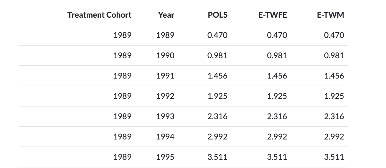
- Bottom line: specify a flexible regression to allow for heterogeneity across time and treatment cohorts.
- For a balanced panel, POLS, TWFE and TWM yield identical DID estimates.
- Allows for extensions into nonlinear DID models.
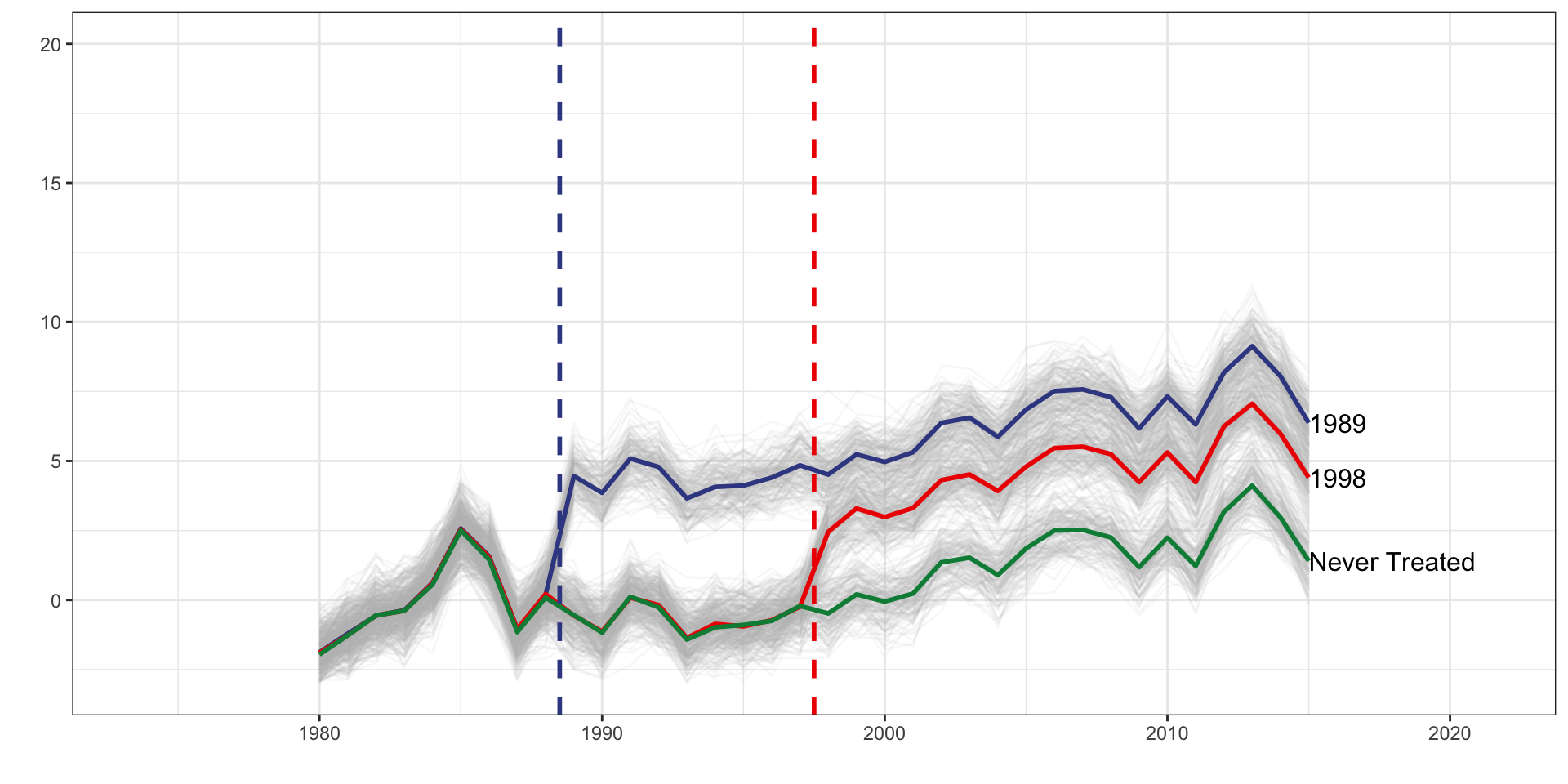
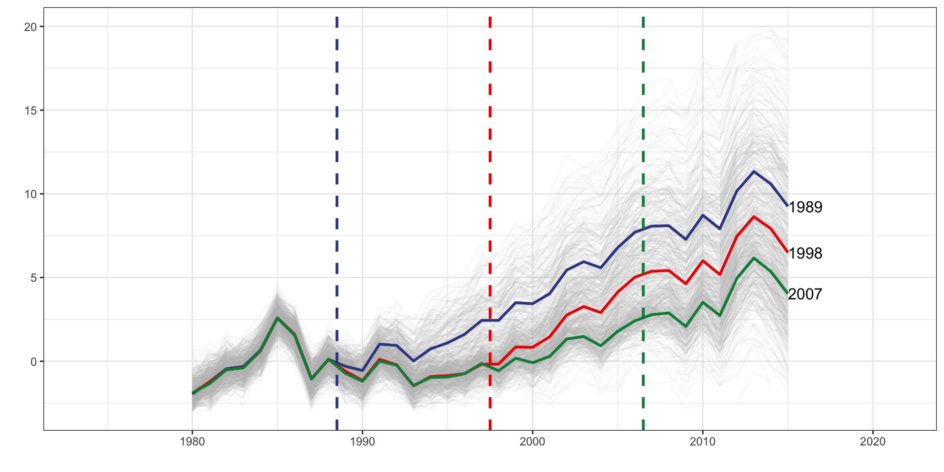
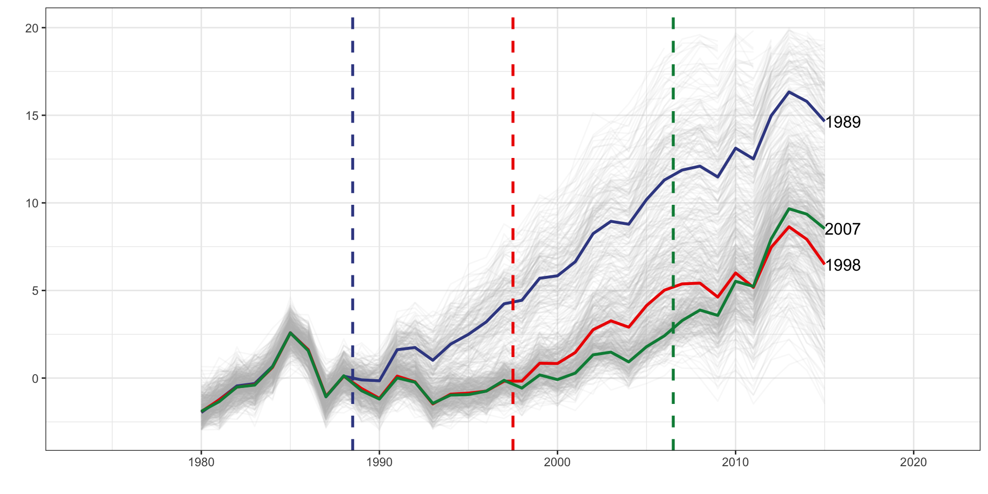
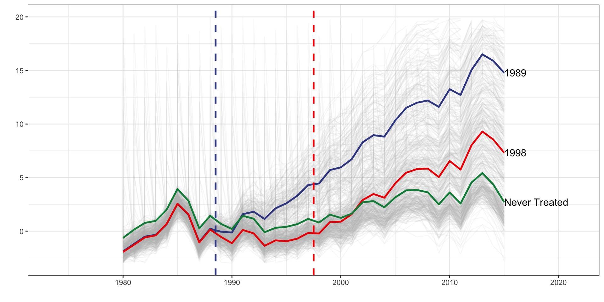
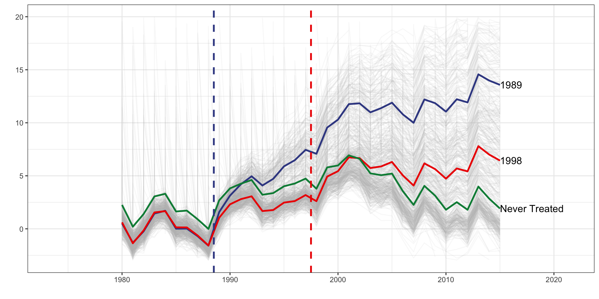
Data Generation Process
Multiple Treatment Periods and Heterogeneous Dynamic Treatment Effects, Never Treated Group
Please Note
DGP code adapted from Baker, Andrew C., David F. Larcker, and Charles CY Wang. “How much should we trust staggered difference-in-differences estimates?.” Journal of Financial Economics 144.2 (2022): 370-395.
Raw Data
| unit |
year |
y_it |
d_it |
x_i |
x_it |
| 1 |
1980 |
0.659 |
0 |
2.666 |
-0.416 |
| 1 |
1981 |
-1.404 |
0 |
2.666 |
1.125 |
| 1 |
1982 |
-0.133 |
0 |
2.666 |
1.001 |
| 1 |
1983 |
1.849 |
0 |
2.666 |
-0.575 |
| 1 |
1984 |
1.833 |
0 |
2.666 |
1.606 |
| 1 |
1985 |
0.661 |
0 |
2.666 |
1.565 |
| 1 |
1986 |
0.508 |
0 |
2.666 |
1.546 |
| 1 |
1987 |
-0.279 |
0 |
2.666 |
3.861 |
| 1 |
1988 |
-2.180 |
0 |
2.666 |
2.276 |
| 1 |
1989 |
0.861 |
1 |
2.666 |
2.653 |
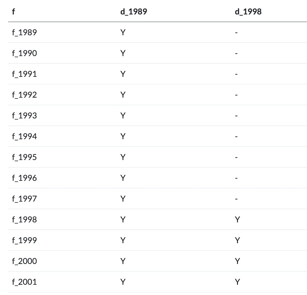
Step 1
![]()
Step 1
- Identify all treatment cohorts based on the first year of treatment.
- Define cohort dummies
d_1989 is a dummy set to one if the unit belongs to the 1989 treatment cohort.d_1998 is a dummy set to one if the unit belongs to the 1998 treatment cohort.
Step 2
![]()
Step 2
- Identify whether there is a never treated comparison group.
- If there is, move to next step.
- If all groups eventually treated:
- We no longer have viable untreated comparisons after the last cohort is treated.
- Identify the treatment year for the last treated cohort.
- Drop all observations with year \(>=\) the last treatment year.
Step 2
- In our example, there is a never treated group.
- This means every treated group has a viable comparator across the entire analytic window.
- Therefore, we don’t need to drop any observations.
Step 3
![]()
Step 3
- Analytic window is 1980 to 2015
- First treated year is 1989.
f_* covers year dummy variables from 1989 to 2015
Step 4
![]()
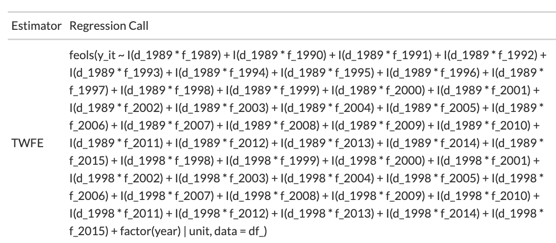
Step 4
- Basic idea is to create interactions between treatment cohort dummies and post-treatment time period dummies.
- For the 1989 cohort, we’d create dummy interactions for
d_1989 * f_1989d_1989 * f_1990d_1989 * f_1991- … and so on.
Step 4
- Basic idea is to create interactions between treatment cohort dummies and post-treatment time period dummies.
- For the 1998 cohort, we’d create dummy interactions for
d_1998 * f_1998d_1998 * f_1999d_1998 * f_2000- … and so on.
Step 4
- In R, you can specify these dummies in the regresison equation using
I(d_1989 * f_1989).
Step 5
![]()
Step 5
| Two-Way Fixed Effects |
feols(I(d* : f*) + factor(time) | unit) |
Unit Fixed Effect |
| Pooled OLS |
lm(I(d* : f*) + factor(time) + d*) |
|
| Two-Way Mundlak |
lmer(I(d* : f*) + factor(time) + d* + (1|unit) |
Unit Random Effect |
Step 5 (with covariates)
See the course blog for how to demean the covariates so they can be included.
| Two-Way Fixed Effects |
feols(I(w : d* : f*) + I(w : d* : f* : x_dm_d*) + factor(time) + I(factor(time) * x_dm_d*) | unit) |
Unit Fixed Effect |
| Pooled OLS |
lm(I(w : d* : f*) + I(w: d* : f* : x_dm_d*) + factor(time) + I(factor(time) : x_dm_d*) + d* + x + I(d* : x_dm_d*)) |
|
| Two-Way Mundlak |
lmer(I(w : d* : f*) + I(w: d* : f* : x_dm_d*) + factor(time) + I(factor(time) : x_dm_d*) + d* + x + I(d* : x_dm_d*) + (1|unit) |
Unit Random Effect |
Regression Call: TWFE
feols(I(d* : f*) + factor(time) | unit)
![]()
Results: Coefficient Estimates
![]()
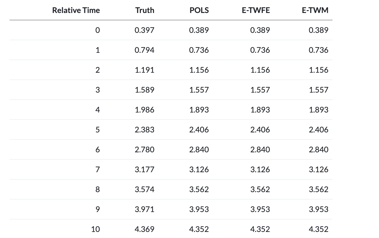
Results: Relative Time
- You can also align each coefficient to its point in relative time.
- For 1989 treated cohort, coefficient on
I(d_1989 * f_1989) corresponds to relative_time=0.
- For 1998 treated cohort, coefficient on
I(d_1998 * f_1998) corresponds to relative_time=0.
Results: Relative Time
- Once you get all treatment effect coefficients organized into relative time, you can take the average (across treated cohorts) at each time period.
- Can plot these effect estimates (analogous to the event study plot from earlier).
Results: Relative Time
![]()
Extended Difference-in-Differences
| Single |
Single |
No |
Constant |
Yes |
Yes |
Yes |
| Single |
Single |
No |
Dynamic |
Yes1 |
Yes |
Yes |
| Multiple |
Single |
No |
Constant |
Yes |
Yes |
Yes |
| Multiple |
Single |
Yes |
Constant |
No |
No |
Yes |
| Multiple |
Staggered |
No |
Constant |
No |
Yes |
Yes |
| Multiple |
Staggered |
Yes |
Constant |
No |
No |
Yes |
| Multiple |
Single |
No |
Dynamic |
No |
No |
Yes |
| Multiple |
Single |
Yes |
Dynamic |
No |
No |
Yes |
| Multiple |
Staggered |
No |
Dynamic |
No |
No |
Yes |
| Multiple |
Staggered |
Yes |
Dynamic |
No |
No |
Yes |