Bayes’ Theorem & Probability Revision

Learning Objectives and Outline

Learning Objectives

• Recognize the importance of Bayes’ Theorem within a Decision Analysis context

• Reproduce Bayes’ within context of sensitivity/specificity/positive & negative predictive values

• Solve & revise probabilities using a variation of other methods

• Touch base on lab

• For THIS WEEK’S CLASS, we are going to get into probability revision & Bayes’ Theorem as it pertains to diagnostic testing within decision-making & in the second hour, positivity criterion

Medical Testing

Testing is done for:

• Screening (primary prevention)

• Diagnosis (secondary prevention)

• Monitor and guide treatment (tertiary prevention)

• Prognosis

Keeping Bayes’ Theorem in mind, let’s jump into diagnostic testing & then we will see how we would apply Bayes’ theorem within the context of test results

MEDICAL TESTING is done for –

Screening as it relates to primary prevention EX: HPV screening for cervical cancer prevention

Diagnosis, or secondary prevention EX: Diagnosis of Hepatitis C, which the earlier diagnosis the better in terms of the disease getting worse over time

To monitor & guide treatment (otherwise known as tertiary prevention) EX: Diabetes could be a good example of this – the goal is to improve quality of life by limiting or delaying complications, restoring function, etc.

To make a prognosis EX: The likely course of a disease

Information for decision making

Clinicians have a variety of diagnostic information to guide their decision making

• Talking to patient (history, symptoms)

• Physically examining patient

• Screening (cervical cancer) + diagnostic tests (EKGs, Blood tests, X-rays)

Information for decision making

Obtaining information can be…

• RISKY
  

• EXPENSIVE
  

• ERROR PRONE
  

• ALL THREE

RISKY/INVASIVE – For example, getting an Amniocentesis during pregnancy (A medical procedure used primarily in prenatal diagnosis of chromosomal abnormalities and fetal infections) can significantly increase one’s risk of a miscarriage.

EXPENSIVE – An MRI, for example, is pricey

ERROR PRONE – Diagnostic tests, like anything, aren’t perfect; though, some are more perfect than others

ALL THREE –A diagnostic test, for example, could be all three – risky, expensive, & not very precise

**We need to factor in these tradeoffs when making decisions

Role of Decision Analysis Methods

• Can be used to weigh the costs and benefits:
  • Test costs
  • Test accuracy
  • Health risks of testing

Example: Diagnostic Tests

What is the chance that a patient has a disease if a diagnostic test is positive or negative?

Example: Diagnostic Tests

What is the chance that a patient has a disease if a diagnostic test is positive or negative?

In other words, what is the probability of disease conditional on the test result? (D+ | T+); (D+ | T-)

Ways to get revised (posterior) probabilities

1. Bayes’ theorem
   
2. 2x2 tables
   
3. Bayes’ theorem via decision tree inversion
   
4. Odds/likelihood ratio [extra slides]
   

Ways to get revised (posterior) probabilities

1. Bayes’ theorem
   
2. 2x2 tables
   
3. Bayes’ theorem via decision tree inversion
   
4. Odds/likelihood ratio [extra slides]
   

1. Bayes’ Theorem: Intuition

Population of 200 indiviudals

Disease (red) has 1% prevalence.

A Screening Test is Available

 

 

Test will detect 100% of positive cases.

3% of disease-free individuals will test positive

Eight Positive Tests

 

 

 

Probability of Disease Given Positive Test

 

 

Key Points

• While the test always detects a true case, it also returns false positives.
• The higher the number of false positives, the lower the probability that a given positive result is actually an individual with the disease.

False Positives

• Could be the result of a poor test (e.g., 3% false positive rate).
• Or could be the result of a disease with very low prevalence in a large population, but a very good test!
  • In a population of 200 million, a test with a 0.01% false positive rate will yield 20,000 false positive readings!
  • If the disease prevalence is low (e.g., 0.001%, or 2,000 sick individuals), the probability that someone is sick if they test positive is <10%!

Bayes’ Theorem: Theory

Probability of B

Pr(B)

Probability of A and B

\begin{aligned} Pr(A \& B) &= Pr(A|B) Pr(B)\\ &= Pr(B|A) Pr(A) \end{aligned}

Probability of A Given B

Pr(A|B) = \frac{Pr(A \& B)}{Pr(B)}

A Perfect Test

100% Specificity, <100% Sensitivity

<100% Specificity, 100% Sensitivity

Let’s Lower Disease Prevalence

<100% Specificity, <100% Sensitivity

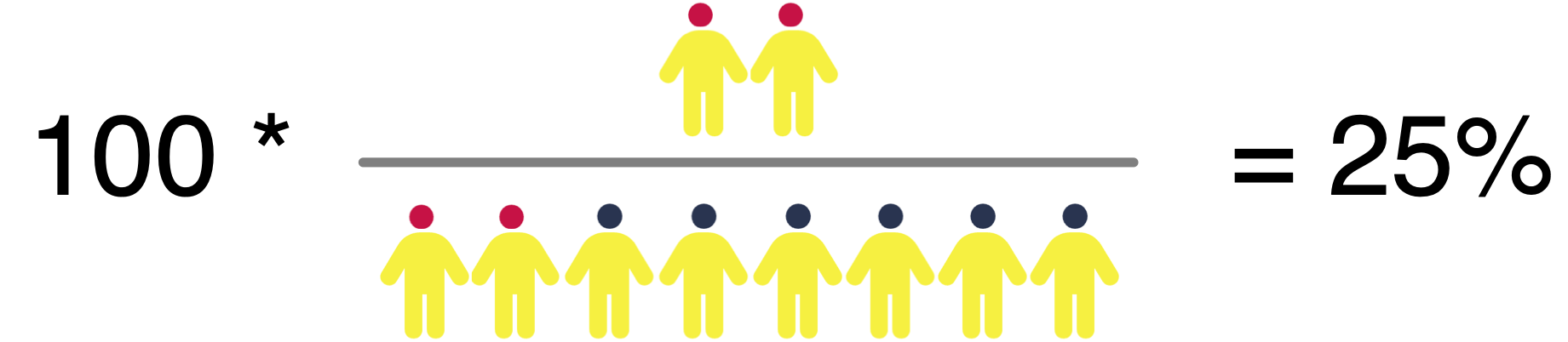
What is the Probability of Disease Given A Positive Test?

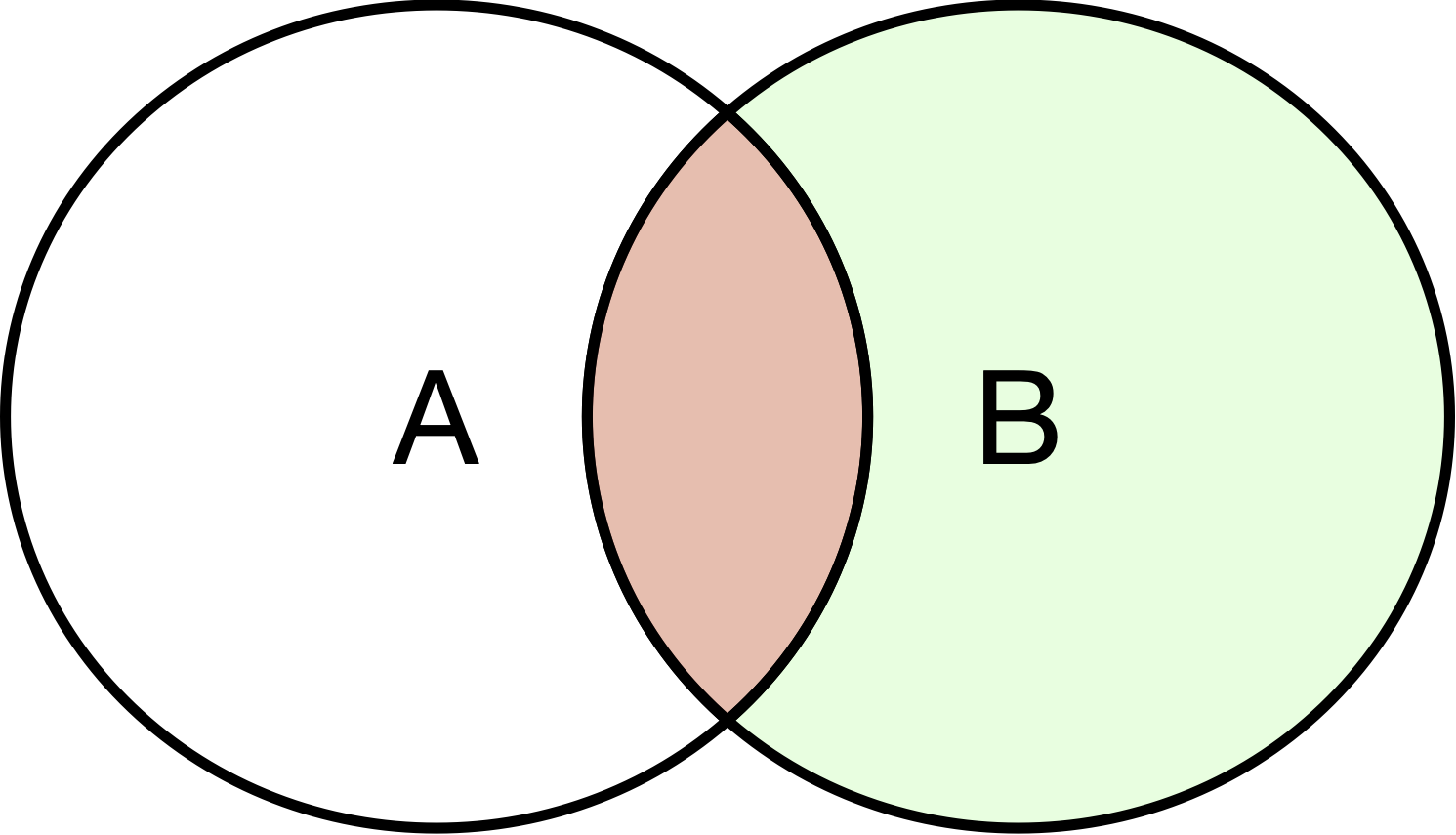
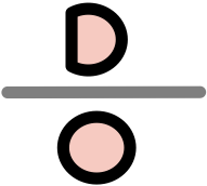
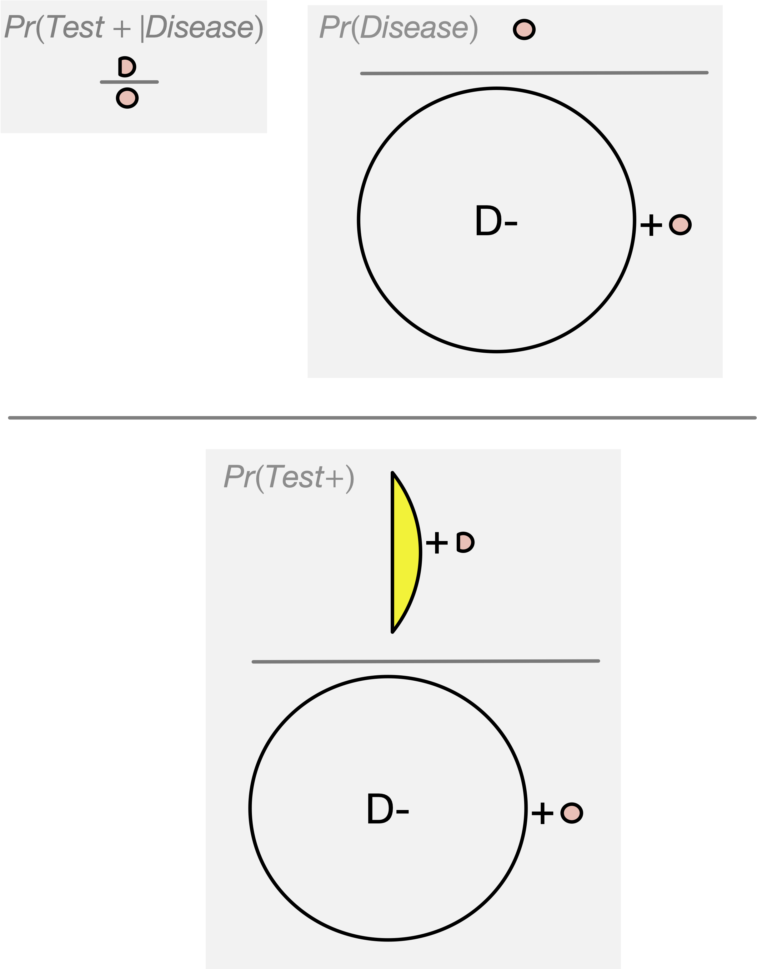
Probability of Testing Positive if Have Disease

 

 

 

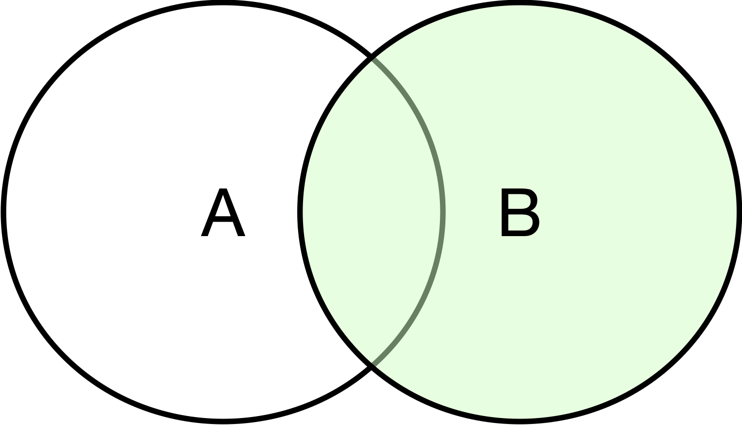
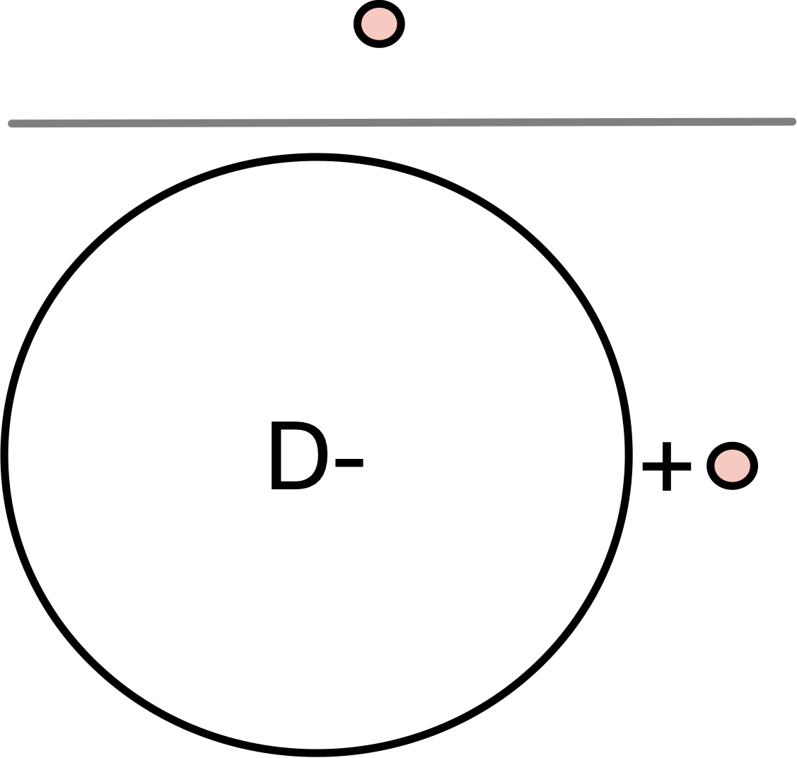
Probability of Having the Disease

 

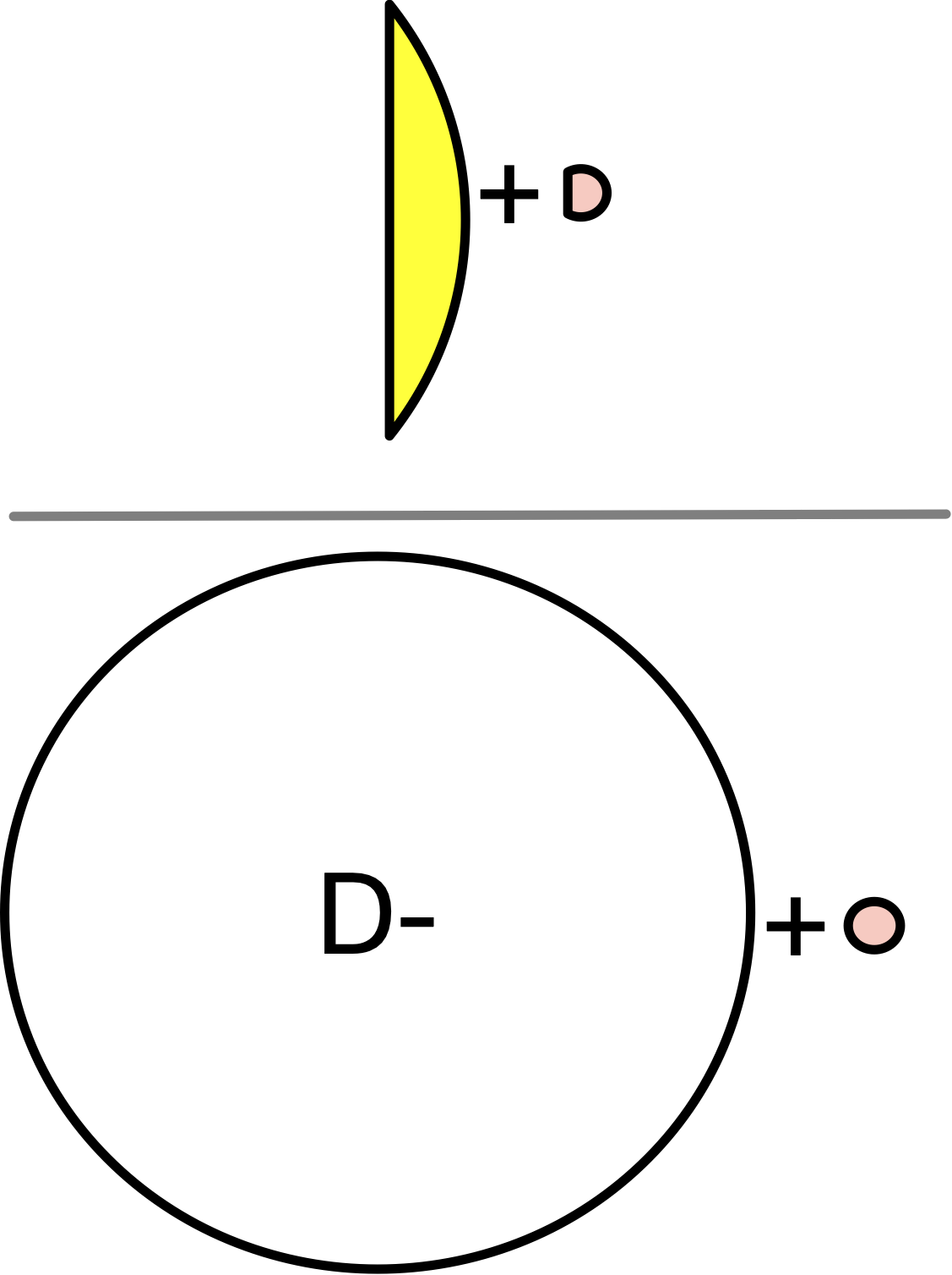
Probability of a Positive Test

 

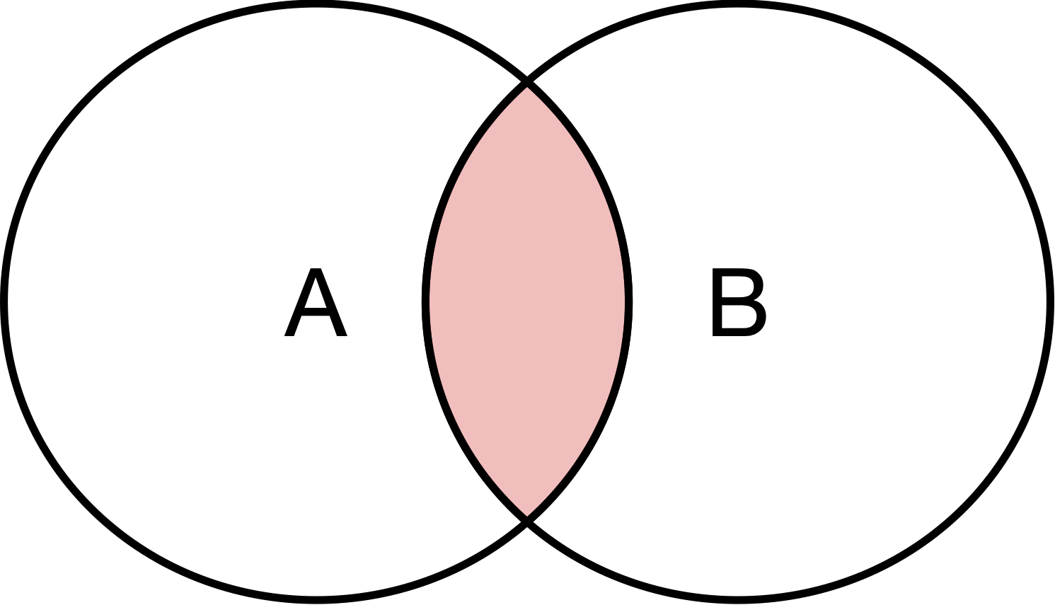
Bayes’ Theorem

 

 

 

1. Bayes theorem describes the probability of an event BASED ON the PRIOR knowledge of conditions that might be related to the event

2. When conducting decision analyses in real life, sometimes, the probability of A given B is easier to get (or vice versa) and you’re not able to find the probability of B given A. So, you can use Bayes’ theorem to convert probabilities into what you need based on the data you have in the real world

3. Conditional probabilities are related according to Bayes’ theorem – in other words, it is a way to RELATE conditional probabilities

4. Explain how to get to Bayes equation*** NOTE: Pr(B) cannot be 0 and Pr(A) cannot be 0 or it becomes undefined

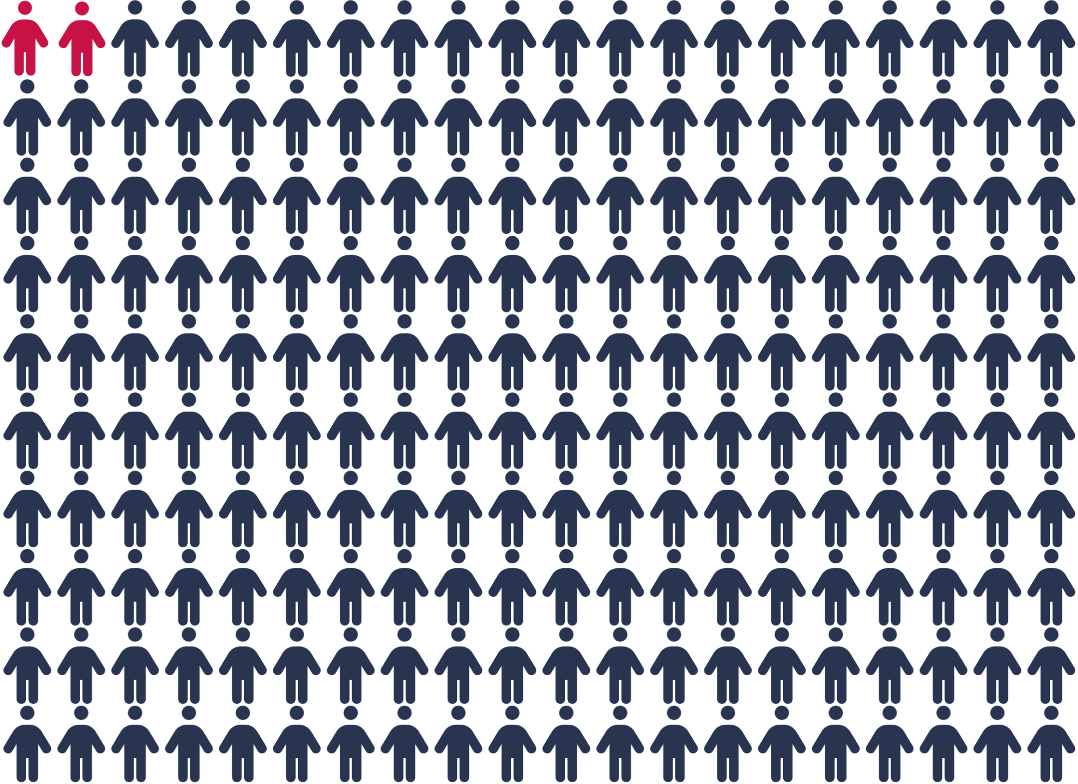
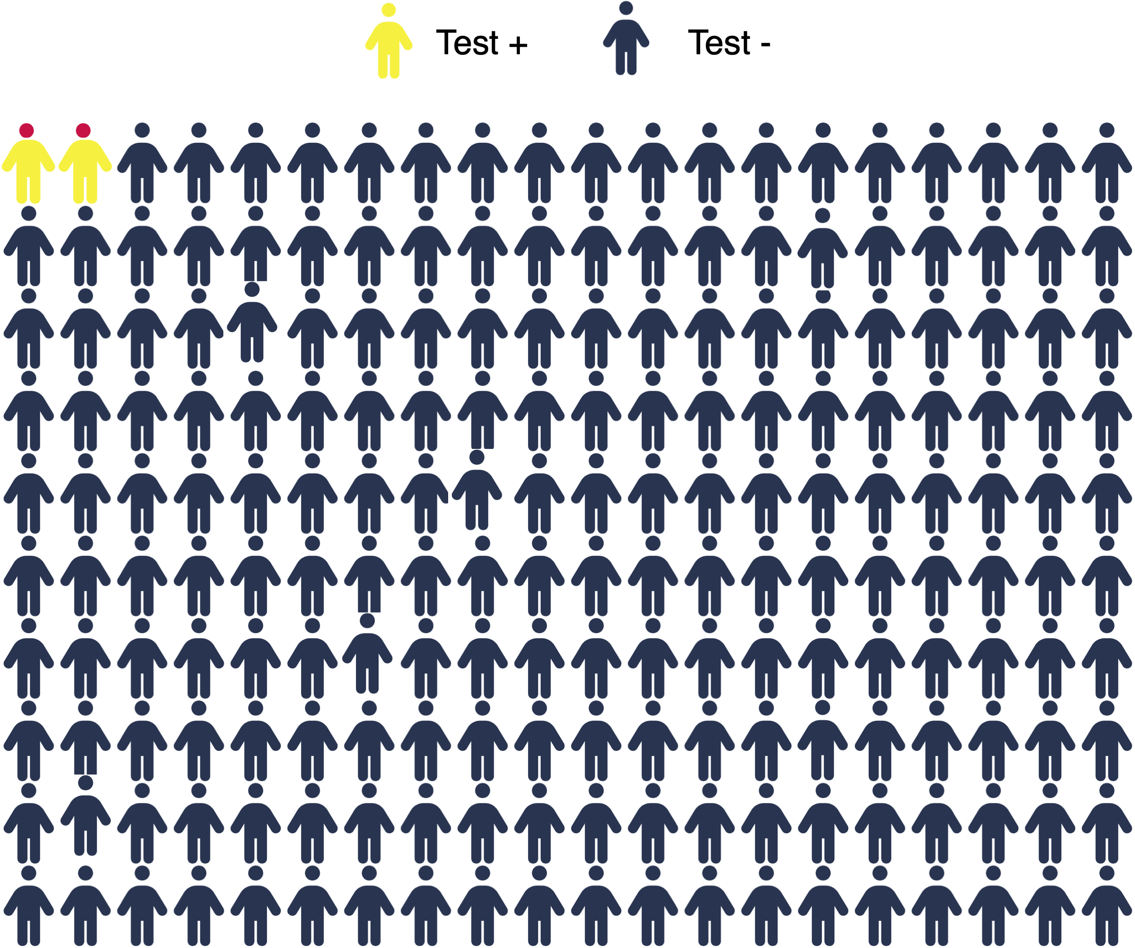
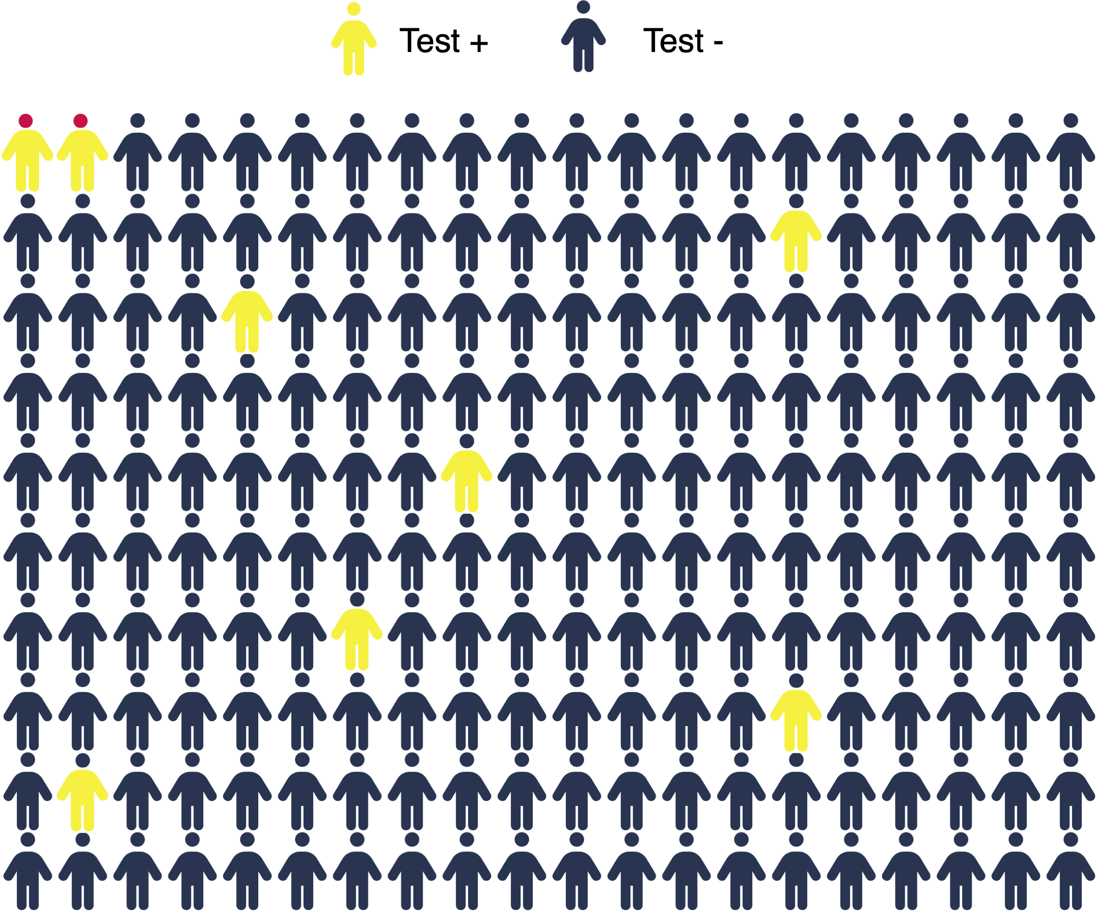
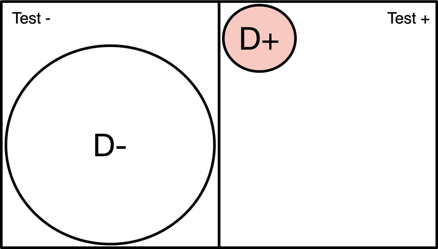
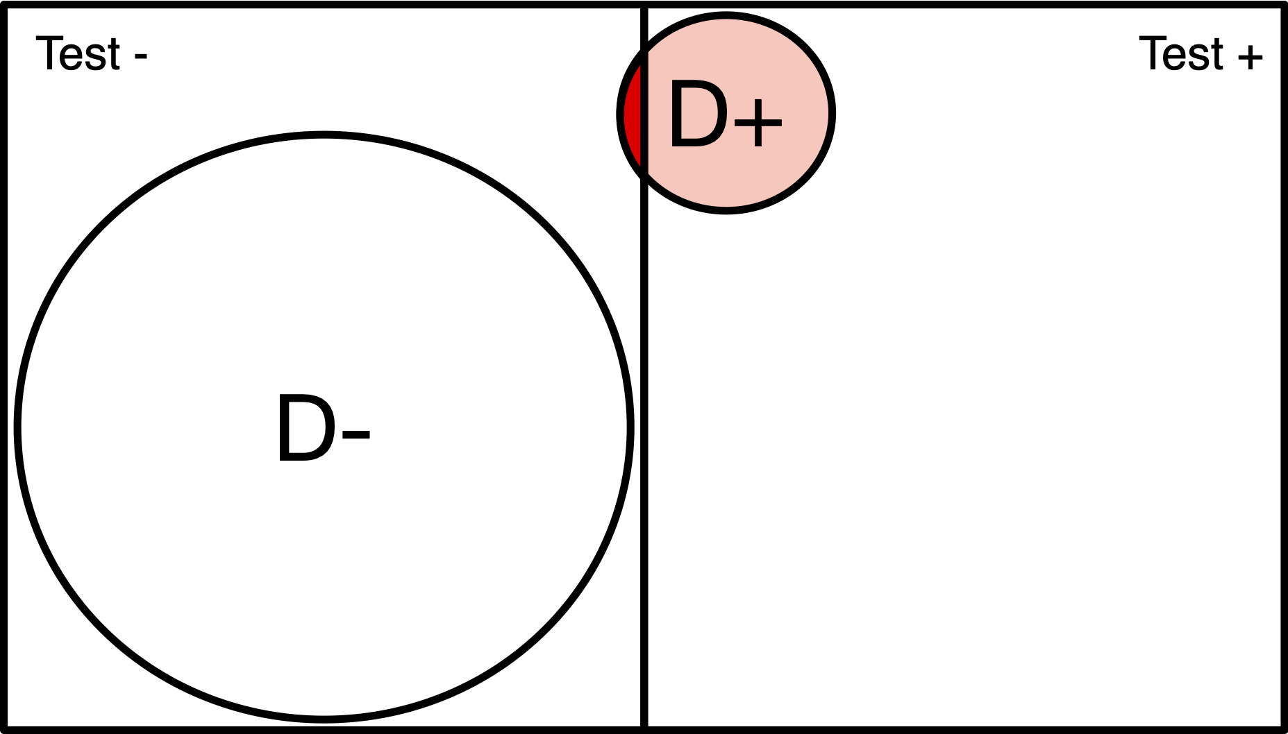
• Population of 200
• Disease (red) has 1% prevalence.
• Test will detect 100% of positive cases.
• 3% of disease-free individuals will test positive

 

 

 

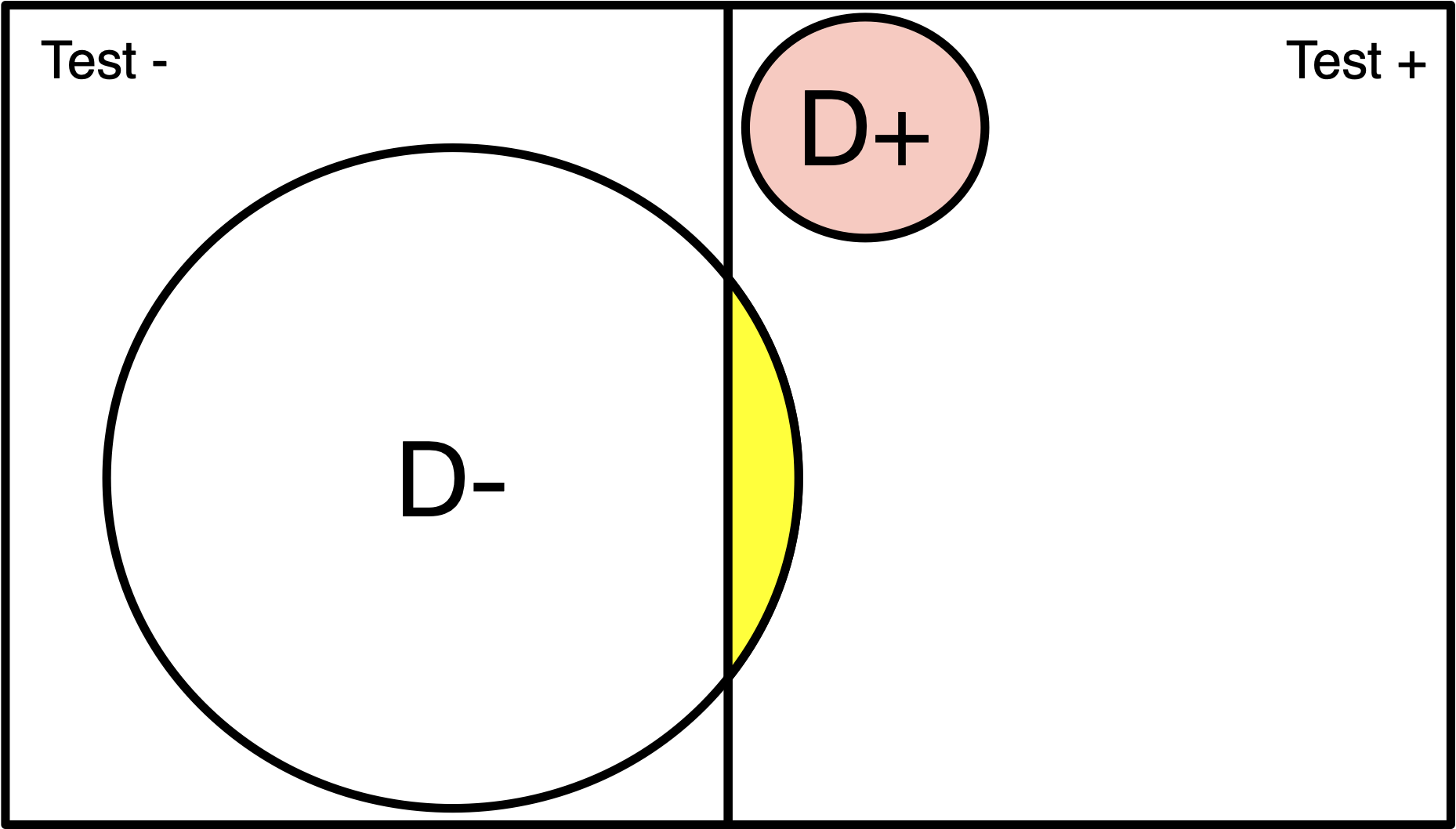
• Population of 200
• Disease (red) has 1% prevalence.
• Test will detect 100% of positive cases.
• 3% of disease-free individuals will test positive

 

 

 

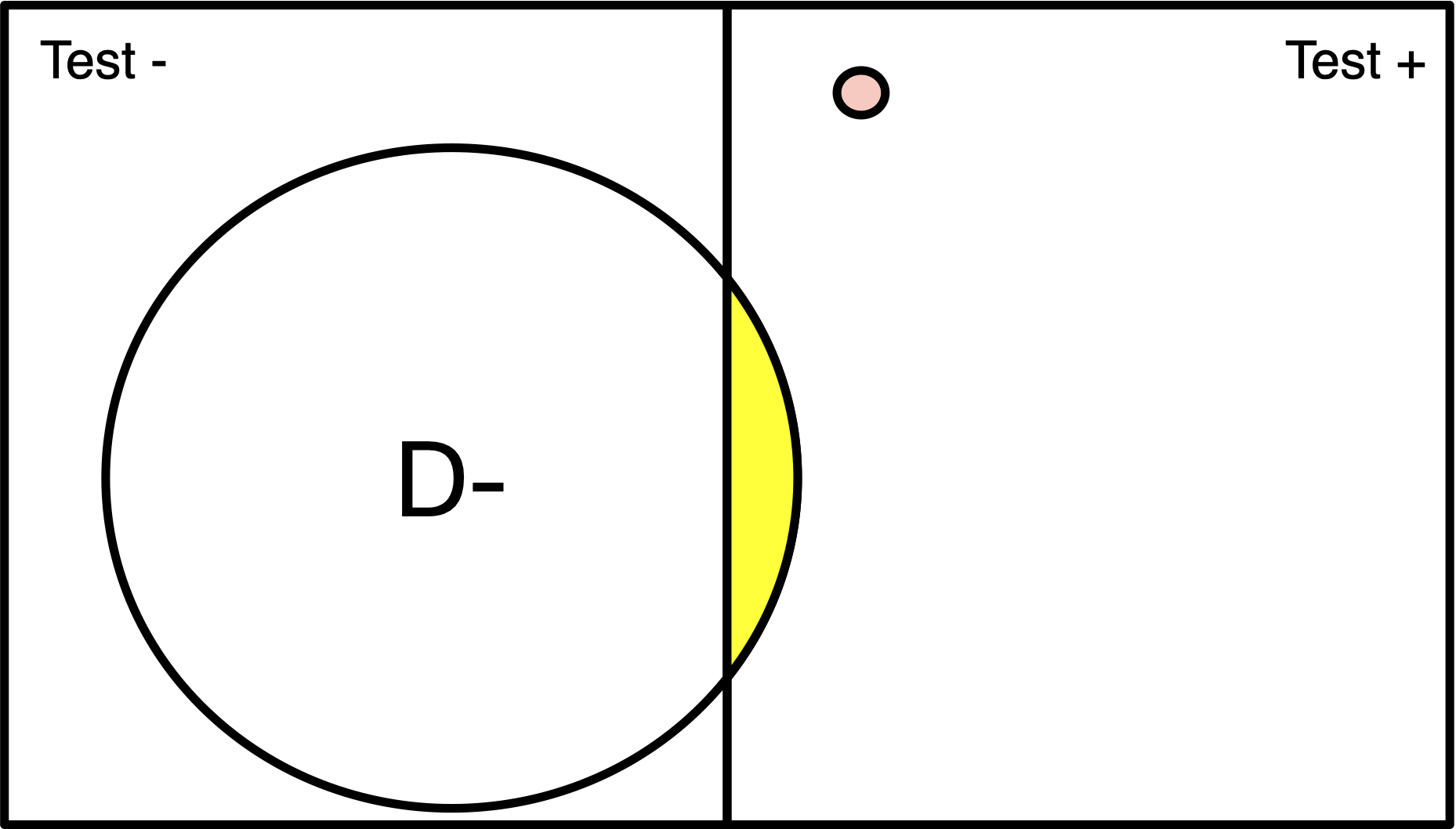
• Population of 200
• Disease (red) has 1% prevalence.
• Test will detect 100% of positive cases.
• 3% of disease-free individuals will test positive

 

 

 

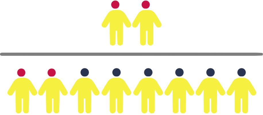
• Population of 200
• Disease (red) has 1% prevalence.
• Test will detect 100% of positive cases.
• 3% of disease-free individuals will test positive

 

 

 

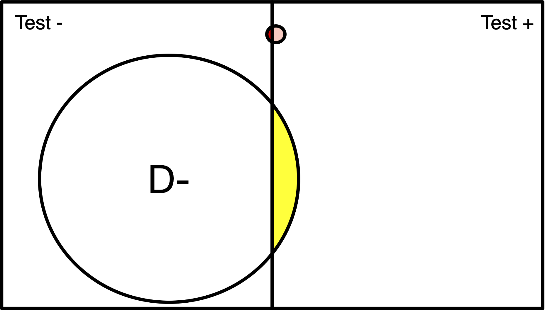
• Population of 200
• Disease (red) has 1% prevalence.
• Test will detect 100% of positive cases.
• 3% of disease-free individuals will test positive

 

 

 

2. 2x2 Tables

2x2 Example: Disease Testing

1. Antibody
   
2. Diagnostic

Let’s look at COVID-19 testing We know that there are two types of tests: Diagnostic & Antibody

Disease Testing

Case example

You are trying to determine what proportion of the population has already been exposed a new communicable disease, in hopes of figuring out if herd immunity is possible.

You decide to do a antibody test to measure the level of antibodies in a sample of 500 participants

Disease Testing

Case example

What is the test’s SENSITIVITY?

What is the test’s SPECIFICITY?

What is the test’s FALSE NEGATIVE RATE?

What is the test’s FALSE POSITIVE RATE?

Disease Testing

Case example

	D+	D-
T+	a (TP)	b (FP)	a + b
T-	c (FN)	d (TN)	c + d
	a + c	b + d	a + b + c + d

One way we can look at these different testing outcomes is through a 2X2 table

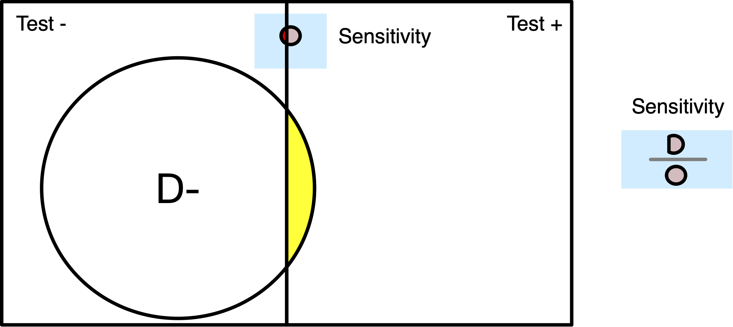
Disease Testing: SENSITIVITY

	D+	D-
T+	125 (a, TP)	20 (b, FP)	145 (a + b)
T-	9 (c, FN)	346 (d, TN)	355 (c + d)
	134 (a + c)	366 (b + d)	500 (a + b + c + d)

Test Sensitivity among those who have or had the virus, 125/134 = 93% (Interpretation: The probability of the screening test correctly identifying diseased subjects was 93%)

1. Sensitivity measures how often a test correctly generates a positive result for people who had the condition that’s being tested for (also known as the “true positive” rate).

2. We would take column A (which is the proportion of people who have a positive COVID antibody test & divide that by everyone who truly had COVID) –

3. As a result, we would get the proportion of people that previously HAD COVID with a TRUE POSITIVE test

(to determine those who “truly” had COVID, the study criteria could have included individuals who had received a range of other confirmatory tests while they had COVID, including lung examinations, other blood work, etc.)

4. For this example, we get a test sensitivity of 93%

5. In other words, a test with 93% sensitivity will correctly return a positive result for MOST people who have had COVID BUT will return a negative result — a false-negative — for 7% of the people who have had COVID & should have tested positive

Disease Testing: SENSITIVITY

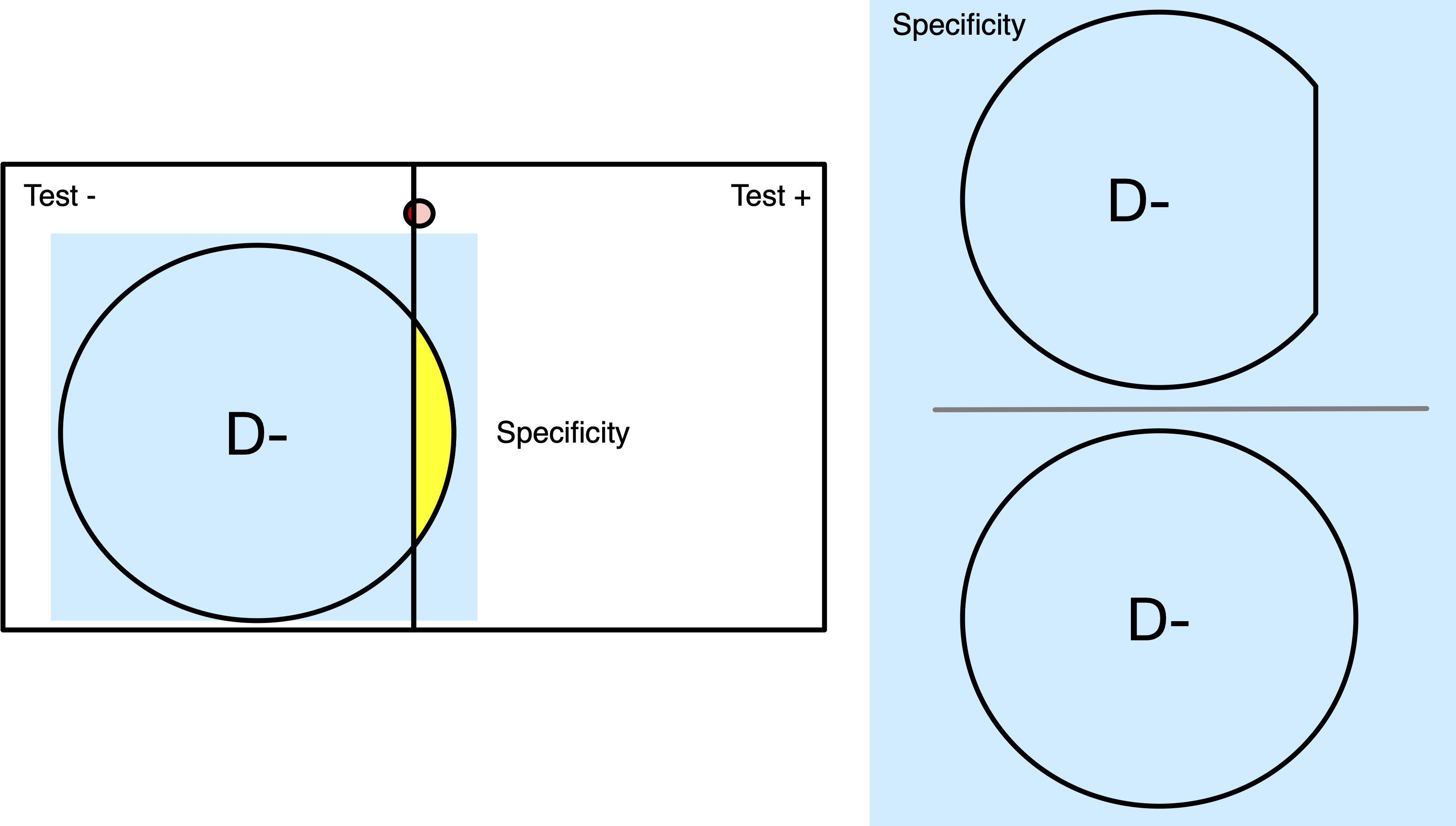
Example: SPECIFICITY

	D+	D-
T+	125 (a, TP)	20 (b, FP)	145 (a + b)
T-	9 (c, FN)	346 (d, TN)	355 (c + d)
	134 (a + c)	366 (b + d)	500 (a + b + c + d)

Test Specificity among those without the disease at any point, 346/366 = 95% (Interpretation: The probability of the screening test correctly identifying non-diseased subjects was 65%)

1. Specificity measures a test’s ability to correctly generate a negative result for people who don’t have the condition (or didn’t have the condition in our case) that’s being tested for (also known as the “true negative” rate).

2. To calculate the SPECIFICITY of the antibody test, we would take column D (which is the proportion of people who tested negative for COVID antibodies & divide that by everyone who truly did NOT have COVID

3. When we do the calculation, the probability of the antibody test correctly identifying those that DID NOT previously have COVID was 95%

4. In other words, a test with 95% specificity will correctly return a negative result for MOST people who didn’t have the disease BUT will return a positive result — a false-positive — for 5% of the people who didn’t have COVID and should have tested negative for the antibodies

Disease Testing: SPECIFICITY

Do you want a test with good Sensitivity or good Specificity?

IT DEPENDS!

EXAMPLE – HIV TEST

If low SENSITIVITY, you have the risk of producing a lot of false-negatives, which could be bad for the population & the spread of the virus + patient not getting the care he/she needs; Not picking up the disease in people who should be picked up

If low SPECIFICITY, there’s an increase risk of false-positive results, which can be devastating & lead to toxicity implications (if you start treatment) + grave emotional consequences + increase healthcare costs Falsely returning positive tests in people that don’t have the disease

False Negatives

False negative rate (1-sensitivity) is the proportion of diseased people with a negative test: c/(a+c)

False Negatives

False negative rate (1-sensitivity) is the proportion of diseased people with a negative test: c/(a+c)

False Negatives

False Positives

False positive rate (1-specificity) is the proportion of non-diseased people with a positive test: b/(b+d)

False Negatives

False positive rate (1-specificity) is the proportion of non-diseased people with a positive test: b/(b+d)

False Negatives

2x2 Example: Disease Testing

1. Antibody
   
2. Diagnostic

Predictive value

…Imagine you are discussing the results of a screening test with a patient

(+) If the patient has an abnormal screening test (i.e. it’s POSITIVE), how likely is it that he really has the disease? [how worried should he be?]

(-) If the test was NEGATIVE, how likely is it that he really does not have the disease? [how reassured should he be?]

Now let’s move to PREDICTIVE VALUE

***Predictive value is especially relevant for screening tests to determine how worried you should be if you have a positive test – in other words, it describes the proportion of people who will go on to have a disease

• If we shift our focus from COVID & think about a screening test that may be predictive of a heart attack, for example: Of those that have a positive test (in other words, indicative of risk for a heart attack), how worried should the patient be in terms of heart attack risk?

• Likewise, of those with a negative test result, what proportion have had heart attacks? – how reassured should you be?

Positive Predictive Value

• Direct application of Bayes’ theorem
• The probability that a person with a positive test result is truly diseased, i.e., Pr(D+|T+)
• Formula:

Positive Predictive Value

• Direct application of Bayes’ theorem
• The probability that a person with a positive test result is truly diseased, i.e., Pr(D+|T+))
• Formula:

\begin{aligned} PPV &=Pr(D+|T+) \\ &= \frac{\text{True Positives}}{\text{True Positives} + \text{False Positives}} \end{aligned}

PPV: How many of test positives are true positives?

Heart Attack:

	Present	Absent
Elevated (+)	300 (a, TP)	15 (b, FP)	315 (a + b)
Normal (-)	35 (c, FN)	150 (d, TN)	185 (c + d)
	335 (a + c)	165 (b + d)	500 (a + b + c + d)

315 patients in this coronary care unit had “elevated” screening levels; out of those 315, 300 had heart attacks. Of those with “elevated” screening levels, what proportion have had a heart attack? PPV = 300/315 = 95%

The denominator here is the TRUE POSITIVE tests as opposed to the TRUE DISEASED like we saw for “sensitivity” In other words, how many of test positives are true positives

• Let’s say we have a hypothetical screening test that can determine HOW LIKELY a patient will develop a heart attack

• And let’s say we do this screening test on 500 patients within a coronary care unit

• 315 patients in this coronary care unit had elevated screening levels predictive of a heart attack Of those 315, 300 had heart attacks, or 95%

5. How worried should a patient be that he will have a heart attack? – pretty concerned, right?

6. ***It’s important to note that as the prevalence of the disease increases, the PPV also increases but the NPV decreases.

The important thing to remember is that PPV (and NPV) show how likely a new assay test result is correct within a population of interest.

Negative Predictive Value

• Direct application of Bayes’ theorem
• The probability that a person with a negative test result is truly non-diseased, i.e., Pr(D-|T-))

Negative Predictive Value

• Direct application of Bayes’ theorem
• The probability that a person with a negative test result is truly non-diseased, i.e., Pr(D-|T-))
• Formula:

\begin{aligned} \text{NPV} &= Pr(D-|T-) \\ &= \frac{\text{True Negatives}}{\text{True Negatives} + \text{False Negatives}} \end{aligned}

NPV: How many of test negatives are true negatives?

	Present	Absent
Elevated (+)	300 (a, TP)	15 (b, FP)	315 (a + b)
Normal (-)	35 (c, FN)	150 (d, TN)	185 (c + d)
	335 (a + c)	165 (b + d)	500 (a + b + c + d)

185 patients in this coronary care unit had normal screening levels; out of those 185, 150 did not have heart attacks. Of those with “normal” screening levels, what proportion did not have heart attacks? NPV = 150/185 = 81%

• Alternatively, we can also calculate the NEGATIVE PREDICTIVE VALUE, i.e. how many of test negatives are true negatives

• For our example, of those with the negative hypothetical screening test, what proportion DID NOT have a heart attack

• In this example: 185 patients in this coronary care unit had NORMAL screening levels Of those 185, 150 did not have heart attacks, or 81%

3. How reassured should a patient be that he will NOT HAVE a heart attack? (“19% worried”)

Predictive values

• Predictive values are highly dependent on the prevalence of disease in a sample (whereas prevalence theoretically should NOT impact sensitivity or specificity)

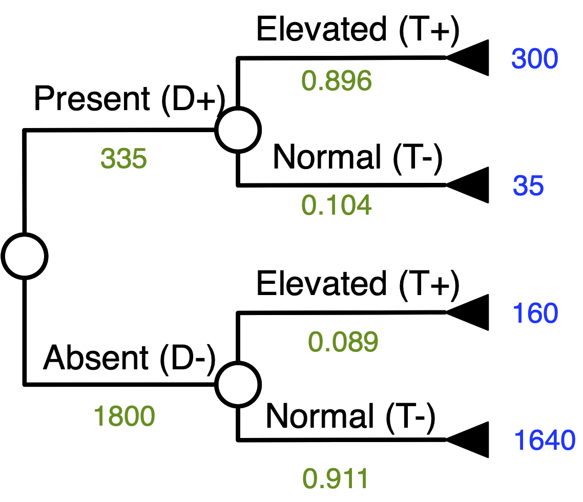
• Previously, we had a population of 500 patients in a coronary care unit, most of whom were having heart attacks.

• Now, let’s switch to a different sample

  - Around 2,100 patients are coming into the ER with chest pain, but most don’t have heart attacks (slightly over 15% have heart attacks)

1. As I had mentioned, predictive values are highly dependent on the prevalence of disease in a sample – they intend to show how likely a new assay test result is correct within a population of interest ***

2. Previously…

3. Now, let’s switch to a different sample just to illustrate this point

Different sample…

	Present	Absent
Elevated (+)	300 (a, TP)	160 (b, FP)	460 (a + b)
Normal (-)	35 (c, FN)	1640 (d, TN)	1675 (c + d)
	335 (a + c)	1800 (b + d)	2135 (a + b + c + d)

When we have a different sample, one that has less disease, the PPV falls & the NPV goes up

Before:

	Present	Absent
Elevated (+)	300 (a, TP)	15 (b, FP)	315 (a + b)
Normal (-)	35 (c, FN)	150 (d, TN)	185 (c + d)
	335 (a + c)	165 (b + d)	500 (a + b + c + d)

If we re-calculate the PPV & NPV within this new population, There are many more people in this sample that are NOT having heart attacks

• The PPV falls and NPV goes up

Different sample…

PPV = 300 / 460 (460 people with “elevated levels” in this sample, only 300 of them are having heart attacks) = 65% (95% in previous sample)

NPV = 1,640 / 1,675 (Of those with “normal levels,” most are not having heart attacks) = 98% (81% in previous sample)

Therefore, the positive & negative predictive values have changed drastically – with the PPV falling to 65% and NPV going up to 98%

2. If we calculate the sensitivity & specificity again, we will see that they are the SAME as before

GOING BACK A SLIDE (3) In the Heart Attack Absent group, there’s a lot of them who are having elevated screening levels (160 now, 15 before) –> NOT BECAUSE the specificity is different, but because there are more non-heart attack patients in this group.

• The PPV here decreases because there will be more false positives for every true positive***

PPV / NPV

On a screening test, a high PPV is acceptable, implying that false positive outcomes are minimized, under a variety of circumstances:

1. When, relative to potential benefits, the costs are high (time/personnel/inconvenience/anxiety/discomfort)
2. Risk of harm from follow-up diagnoses or therapy (such as infection) is high despite the benefits from treatment also being high

Reference: Trevethan (2017)

PPV / NPV

A moderate PPV is acceptable when:

1. False positive outcomes might be “okay” if follow-up tests are inexpensive, easily and quickly performed, and not stressful for clients.
2. If no harm is likely to be done to clients in protecting them against a target condition even if that condition is not present

Reference: Trevethan (2017)

PPV / NPV

A high NPV is acceptable, implying that false negatives are minimized, under a different set of circumstances:

• Quickly progressing diseases, conditions that are not contagious, or those that require treatment early in its course
  

PPV / NPV

A high NPV is acceptable, implying that false negatives are minimized, under a different set of circumstances:

• Quickly progressing diseases, conditions that are not contagious, or those that require treatment early in its course
  

A moderate NPV could be acceptable when:

1. Condition is not serious or contagious or does not progress quickly
2. Dx of condition is ambiguous and subsequent screening tests can be easily scheduled or the condition is likely to resolve without treatment

Reference: Trevethan (2017)

Prevalence and test characteristics

Generally:

• PPV and NPV are dependent on prevalence (Pre-Test Probability)

• SENS + SPEC are usually not dependent on prevalence (spectrum/case-mix bias)

Prevalence and test characteristics

Generally:

• PPV and NPV are dependent on prevalence (Pre-Test Probability)

• SENS + SPEC are usually not dependent on prevalence (spectrum/case-mix bias)

Spectrum bias – Performance of a test may vary in different clinical settings/different mix of patients

3. BUT if SEN/SPEC does happen to change based on the population or prevalence, then you are probably seeing Spectrum Bias – which refers to the phenomenon that the performance of a diagnostic test may vary in different clinical settings because each setting has a different mix of patients

4. To avert this, investigators should design studies to evaluate tests over all relevant subgroups, and where this is not possible, to be explicit about the case mix in the study sample. Furthermore, GPs should endeavor to know both individual patients and practice populations in terms of demographics and co-morbidities before applying study results to their patients.

Predictive values

The pretest (or prior) probability of disease in the 2x2 table before any testing

= Probability of the presence of the target disease conditional on the available information prior to performing the test under consideration

In other words, the proportion of the total population with the disease: (a+c)/(a+b+c+d). This is disease prevalence

1. Let’s get back into Bayesian theory

2. The pre-test or prior probability of disease BEFORE any testing, is essentially the DISEASE PREVALENCE

Latter sample

	Present	Absent
Elevated (+)	300 (a, TP)	160 (b, FP)	460 (a + b)
Normal (-)	35 (c, FN)	1640 (d, TN)	1675 (c + d)
	335 (a + c)	1800 (b + d)	2135 (a + b + c + d)

Disease Prevalence

= (a+c) / (a+b+c+d) = 335 / 2,135 = 0.16

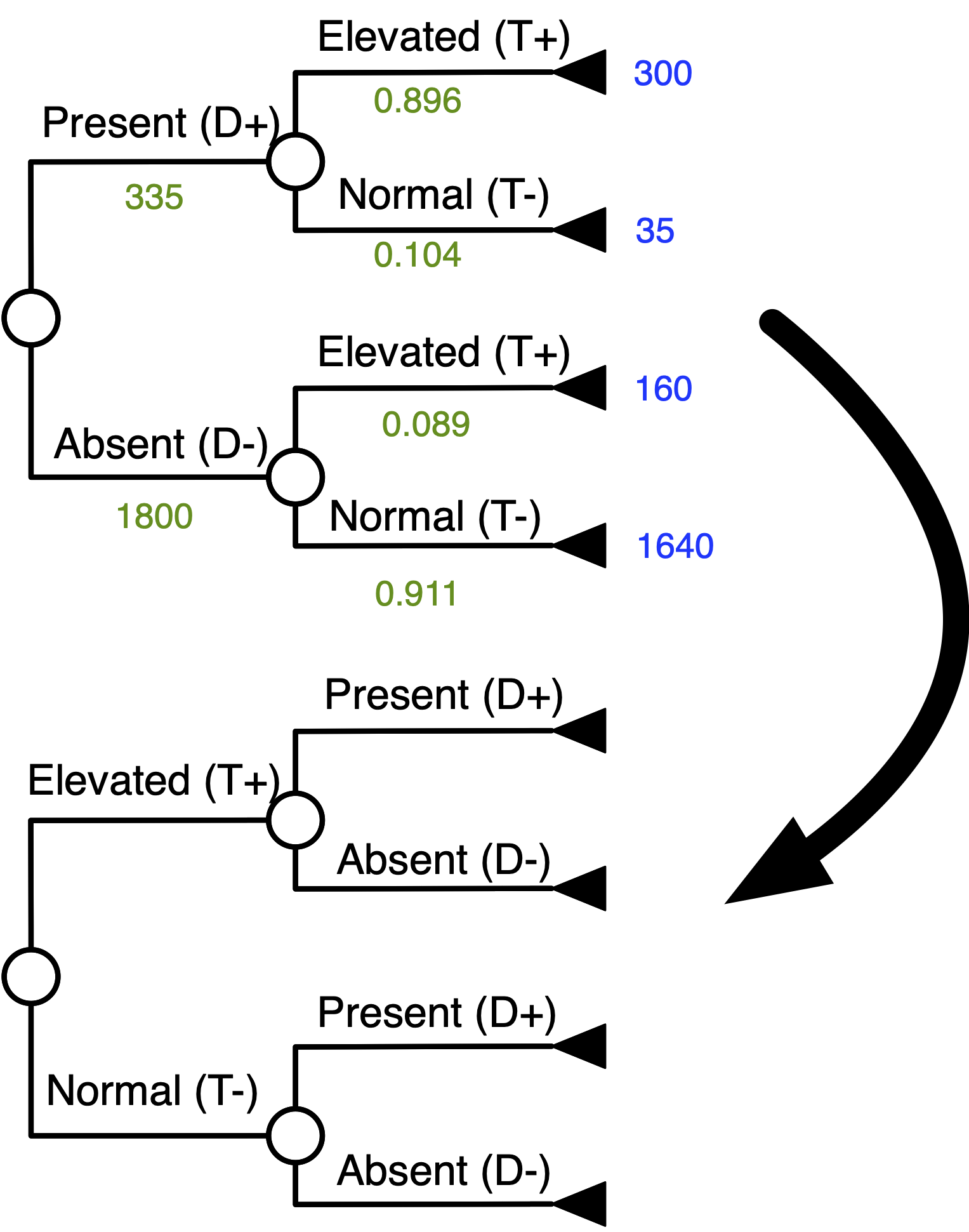
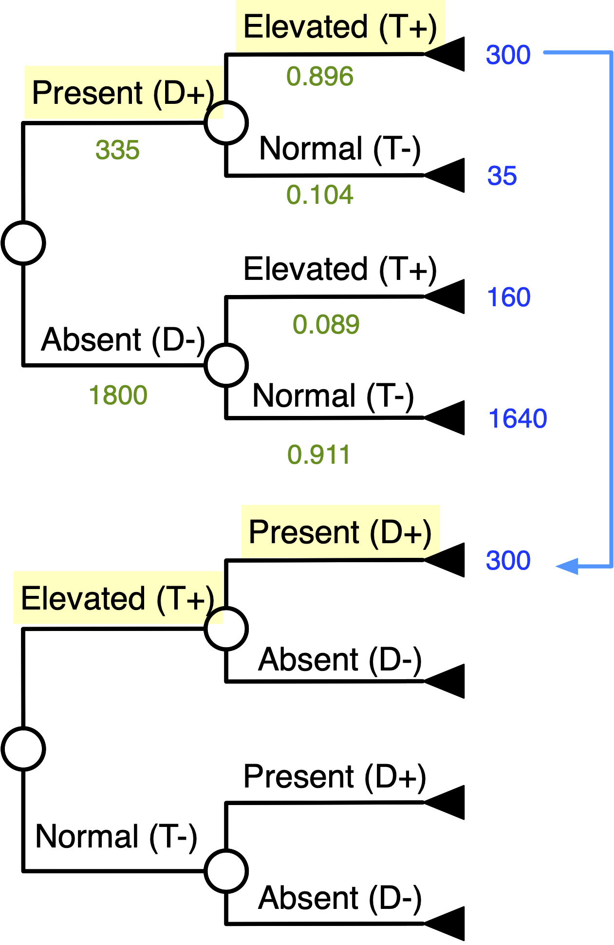
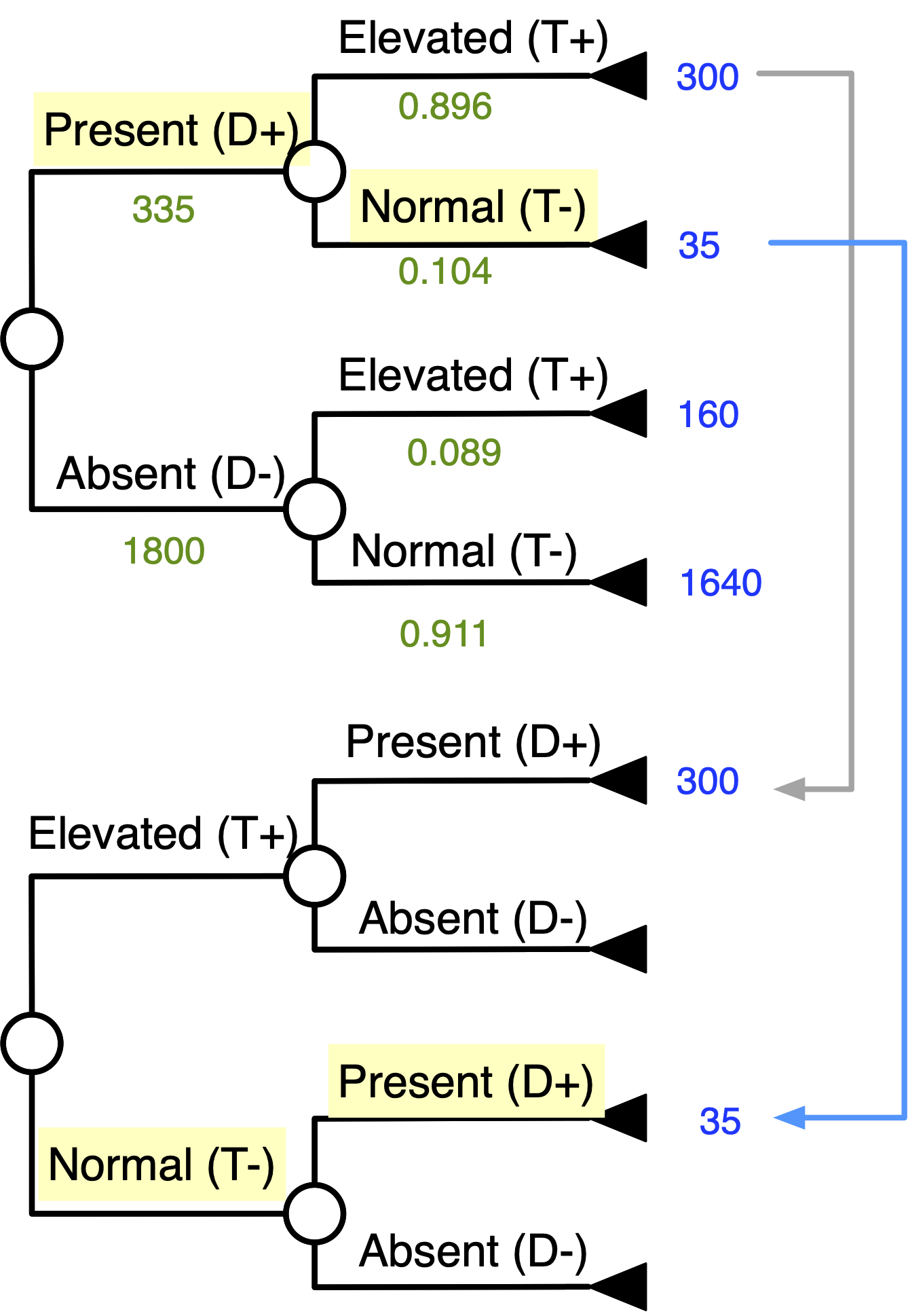
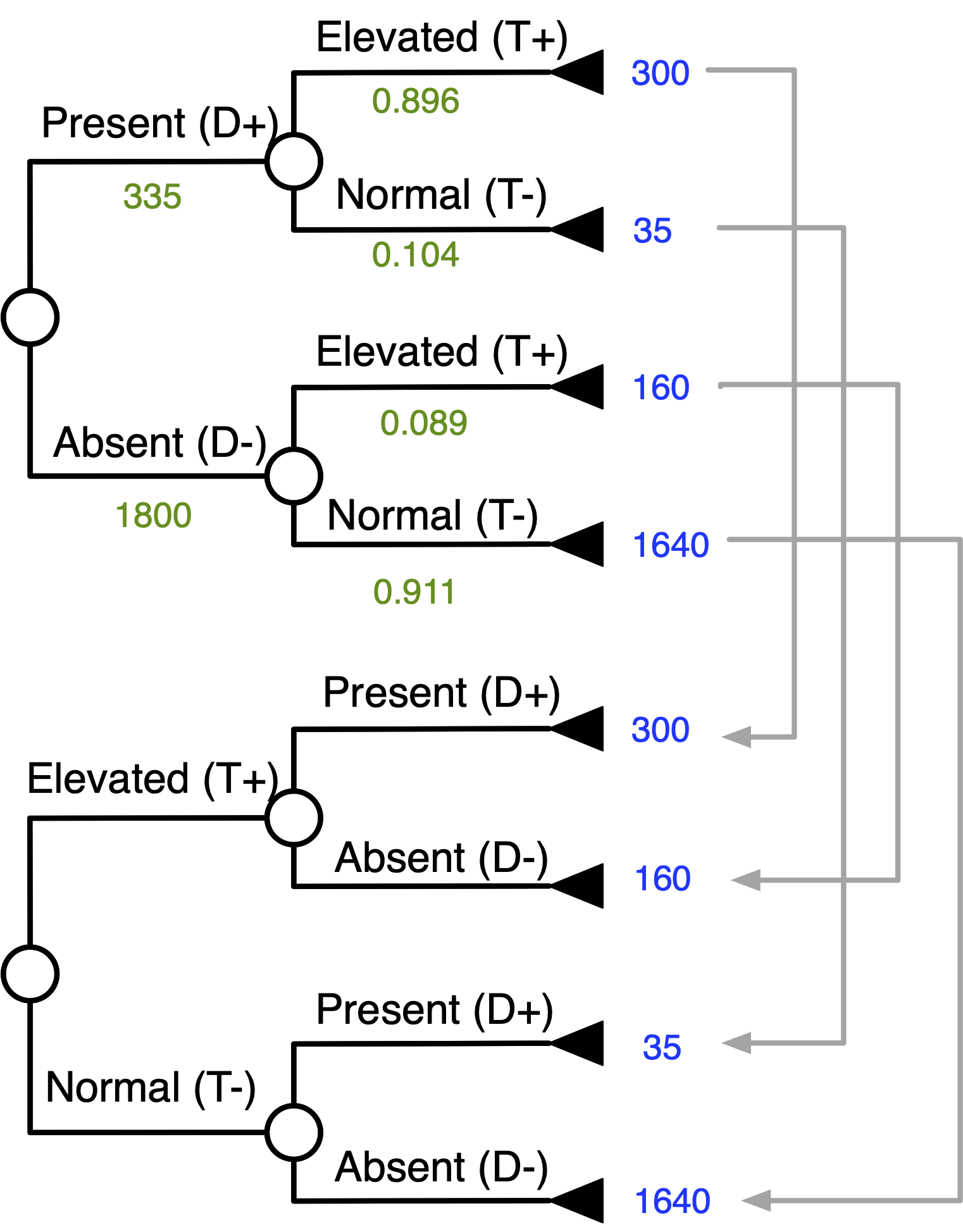
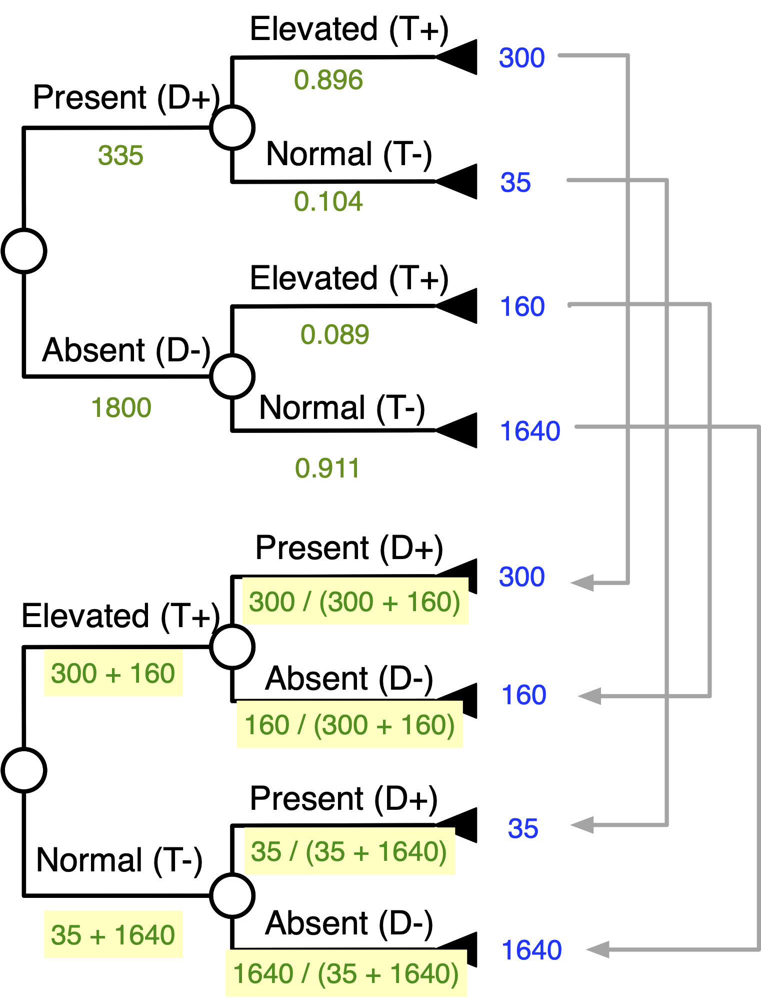
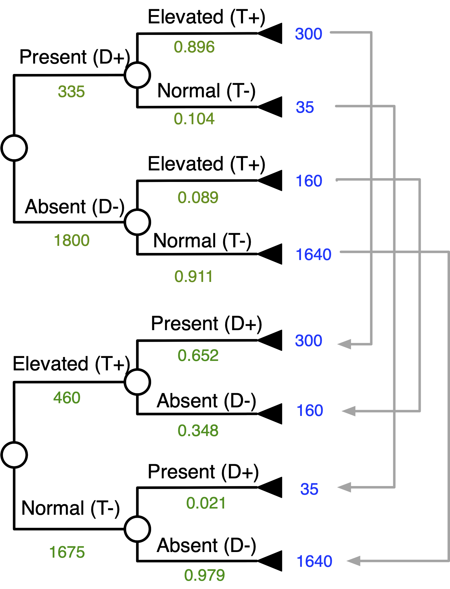
Bayes’ Theorem With Tree Inversion

Bayes’ theorem with tree inversion

• Another way that we can revise probabilities based on the information we have to work with is inverting the tree

• We often have information on the P(T+ | D+) (tree to the right); but mathematically, the tree to the left is the same, but it might be easier to construct the tree this way given the information you have

Goal: “Flip” The Tree

Start Matching Terminal Numbers …

Continue Matching Terminal Numbers …

Continue Matching Terminal Numbers …

Work Your Way Down the Tree …

Inverted Tree

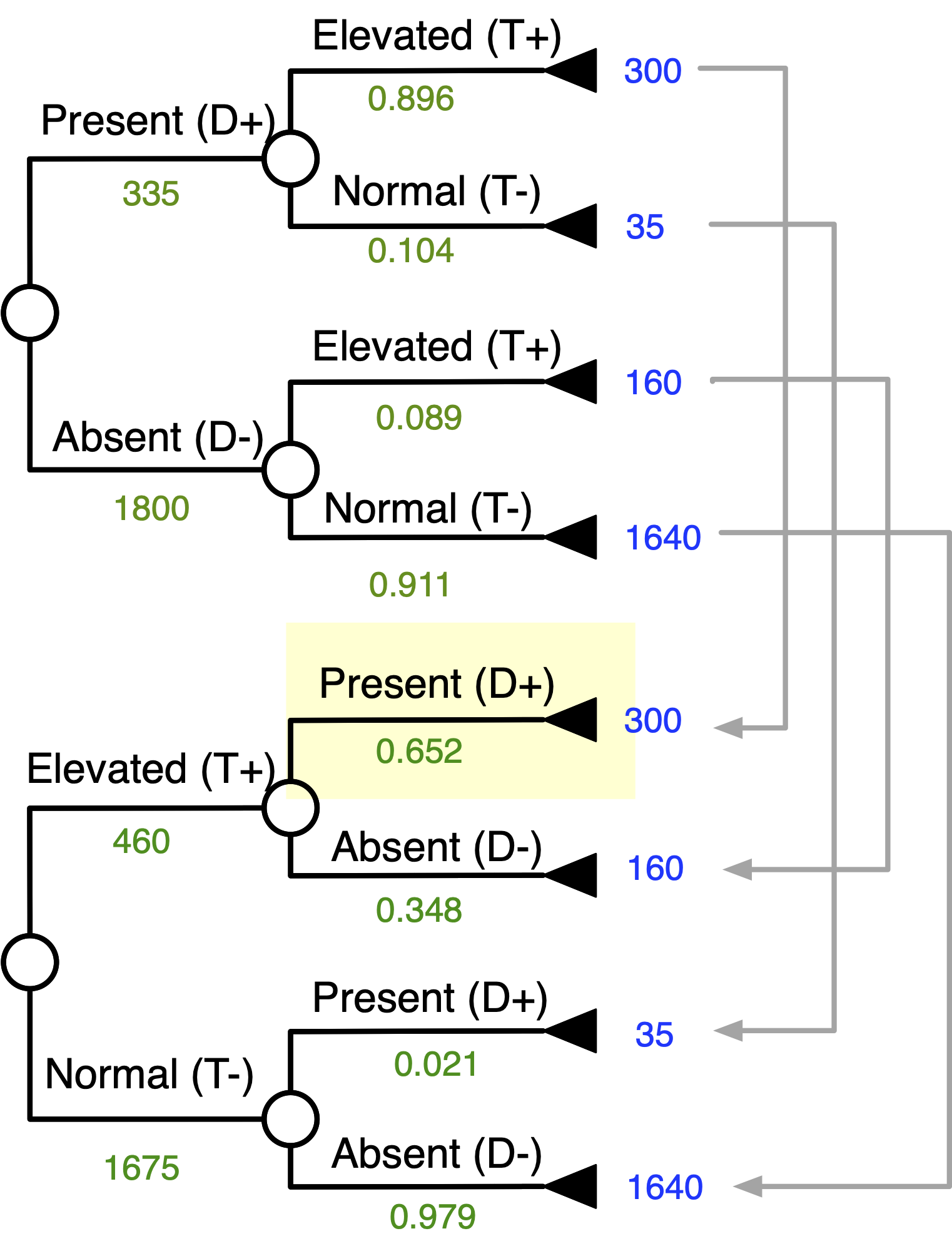
Probability of Disease Given + Test

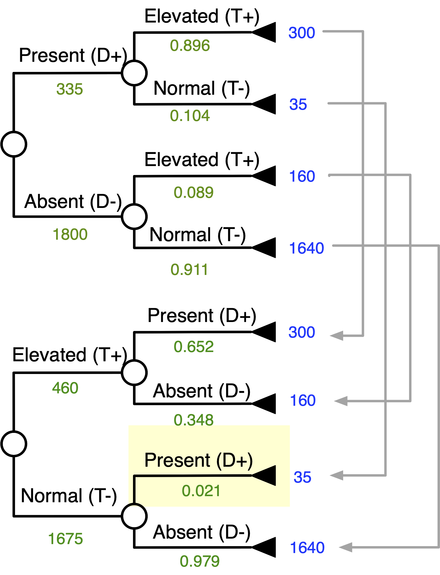
Probability of Disease Given - Test

Conclusions

• We are often bayesian in how we think
• Knowledge of test characteristics can help you to make more informed decisions
• In general, diagnostic tests are helpful when pre-test prob is in the middle (30-70%) and test is going to move you past a decision threshold
• Tests with very good characteristics (ex. 100% sens or spec) can also be very useful if used appropriately

1. You don’t realize it but you’re already thinking about these ratios in your head

• If you’re a surgeon and someone comes in and says that their stomach hurts, you have a certain probability in your mind that they have appendicitis
• Everyday life and other professions – Personality tests, who will benefit from education intervention; Autism screening

2. Pre-test probability is a big deal because you don’t want to do an expensive test with a low pre-test probability, BUT once you find additional information then that can change

[Extra] Likelihood Ratios

Likelihood ratio

Useful for situations in which a quick estimate of revised probabilities is needed

Likelihood that a given test result would be expected in a patient with the target disorder Pr(test result | D+) compared to the likelihood that the same result would be expected in a patient without the target disorder Pr(test result | D-) [A RATIO]

Likelihood ratios

The likelihood ratio (LR) summarizes test sensitivity and specificity into one number:

LR (positive test) = sensitivity/1-specificity (or TPR/FPR)

LR (negative test) = 1-sensitivity/specificity (or FNR/TNR)

Likelihood ratios

• LR can be used to revise disease probabilities using the following form of Bayes’ Theorem:

Post-test odds = Pretest odds x LR

• The odds that the patient has the target disorder, after the test results are known. It is calculated by multiplying the pre-test odds by the likelihood of a positive or negative test.

3. In other words, the post-test odds are the odds that the patient has the target disorder AFTER the test results are known

Likelihood ratios

• LR’s are an advance beyond 2x2 tables

• To use likelihood ratios, you must be comfortable converting between probabilities of disease and odds of disease

• Odds are simply another way of describing the chances that something will (or won’t) happen

Likelihood ratios

Odds of Disease = \frac{\text{Probability}}{\text{1 - Probability}}

Probability = \frac{\text{Odds}}{\text{Odds + 1}}

Likelihood ratios

Odds favoring an event; Odds = p/(1-p) If an event has 0.20 probability of occurrence, the odds favoring the event = 0.2/0.8 = 0.25 (or 1:4)

Odds against (OddA) the event; OddA = (1-p)/p The odds against are 0.8/0.2 = 4 (or 4:1)

The components of the LR are calculated vertically, and like the sensitivity and specificity are immune to the prevalence

Back to first example (coronary care unit)

	Present	Absent
Elevated (+)	300 (a, TP)	15 (b, FP)	315 (a + b)
Normal (-)	35 (c, FN)	150 (d, TN)	185 (c + d)
	335 (a + c)	165 (b + d)	500 (a + b + c + d)

• Pre-test probability was 67% (prevalence)
• SENS = 0.90 & SPEC = 0.91
• LR+ (for positive test result) = SENS / 1=SPEC = 0.90/1-0/.91 = 10
• Interpretation: A patient with a positive test result is 10X more likely to have had a heart attack than someone who did not have a heart attack with the same test result

1. Let’s go back to our 1st example when we were looking at a coronary care unit population
2. The pre-test probability was 67%
3. Sensitivity was 90% & specificity was 91%
4. The Likelihood ratio for a positive test result would be, SENS / 1-SPEC (or, true positive divided by false positives) = 10 This means…

Back to first example (coronary care unit)

• LR - (for a negative test result):
  • 1-SENS / SPEC = 1-0.90 / 0.91 = .11, indicates a ~10-fold decrease in the odds of having a condition in a patient with a negative test result.

1. The Likelihood ratio for a NEGATIVE test result would be, (false negative tests / true negative)

Back to first example (coronary care unit)

Pre-test probability

Pre-test odds (0.67 / 1-0.67)

Post (+ test) odds of disease = pre-test odds * LR(+)

Post (+ test) prob of disease = post-test odds / post-test odds + 1

Post (- test) odds of disease = pre-test odds * LR(-)

Post (- test) prob of disease = 0.22 / 1.22

1. Now let’s calculate the pre & post-test ODDS using what we found the LR’s to be

2. Pre-test odds = Prob / 1-Prob = 2 ; In other words, [2:1] - If you play the game 3 times, you’re likely to win twice

3. Post-test odds = pre-test odds * LR

• Post-test odds of a POSITIVE test = 2*10 (10 is the value we got a couple slides back) = 20 ; or 20-fold increase in odds

• Post-test probability of a POSITIVE test = 95%, which is the probability that your patient will have a heart attack given his/her screening test results (worthwhile diagnostic test)

• Post-test odds of a NEGATIVE test = 0.22; 20-fold decrease in odds of having a heart attack in a patient with a negative test result

• Post-test probability of a NEGATIVE test = 18% ; in other words, of those with normal levels, there is an 18% prob that your patient WILL HAVE a heart attack given the negative screening results

Odds Likelihood Form of Bayes

Odds LR = \frac{\text{Pr(D+ | test result)}}{\text{Pr(D- | test result)}} = \frac{{Pr(D+)}}{Pr(D-)} * \frac{{lr(D+)}}{lr(D-)}

\frac{{Pr(D+)}}{Pr(D-)} * \frac{{lr(D+)}}{lr(D-)}

The above is the same as:

\frac{\text{Pr(D+ | test result)}}{\text{Pr(D- | test result)}}

Odds Likelihood Form of Bayes

Odds LR = \frac{\text{Pr(D+ | test result)}}{\text{Pr(D- | test result)}} = \frac{{Pr(D+)}}{Pr(D-)} * \frac{\text{Pr(test result | D+)}}{\text{Pr (test result | D-)}}

Pre-test odds favoring disease (the prior):

\frac{{Pr(D+)}}{Pr(D-)}

The post-test odds given the test result:

\frac{\text{Pr(D+ | test result)}}{\text{Pr(D- | test result)}}

Odds Likelihood Form of Bayes

\frac{\text{Pr(test result | D+)}}{\text{Pr (test result | D-)}} = \frac{{Pr(D-)}}{{Pr (D+)}} * \frac{{(CTN - CFP)}}{(CTP - CFN)}

How to calculate an optimal “cut-off” for a test with categorical or continuous results at the point in which we will optimize the cut-off conditional on the (1) prior probability of disease and (2) the consequences of the scenario we are assessing

Next lecture: Positivity Criterion!

• You won’t be tested on this equation, but this is another way of getting the OPTIMAL CUT-OFF VALUE for a continuous or categorical test – remember this for the next lecture on positivity criterion.

• Need to factor in the “interventions/treatment” for the “consequences of false positive” and “consequences of false negative”

Likelihood ratios

LR (+)
GT 10 Excellent
5-10 Good
2-5 Fair. May be helpful
1-2 Unlikely to be helpful

LR (-)
<0.1 Excellent
0.1-0.2 Good
0.2-0.5 Fair. May be helpful
0.5-1.0 Unlikely to be helpful

1. The higher diagnostic odds ratios are indicative of better test performance, which you can see here