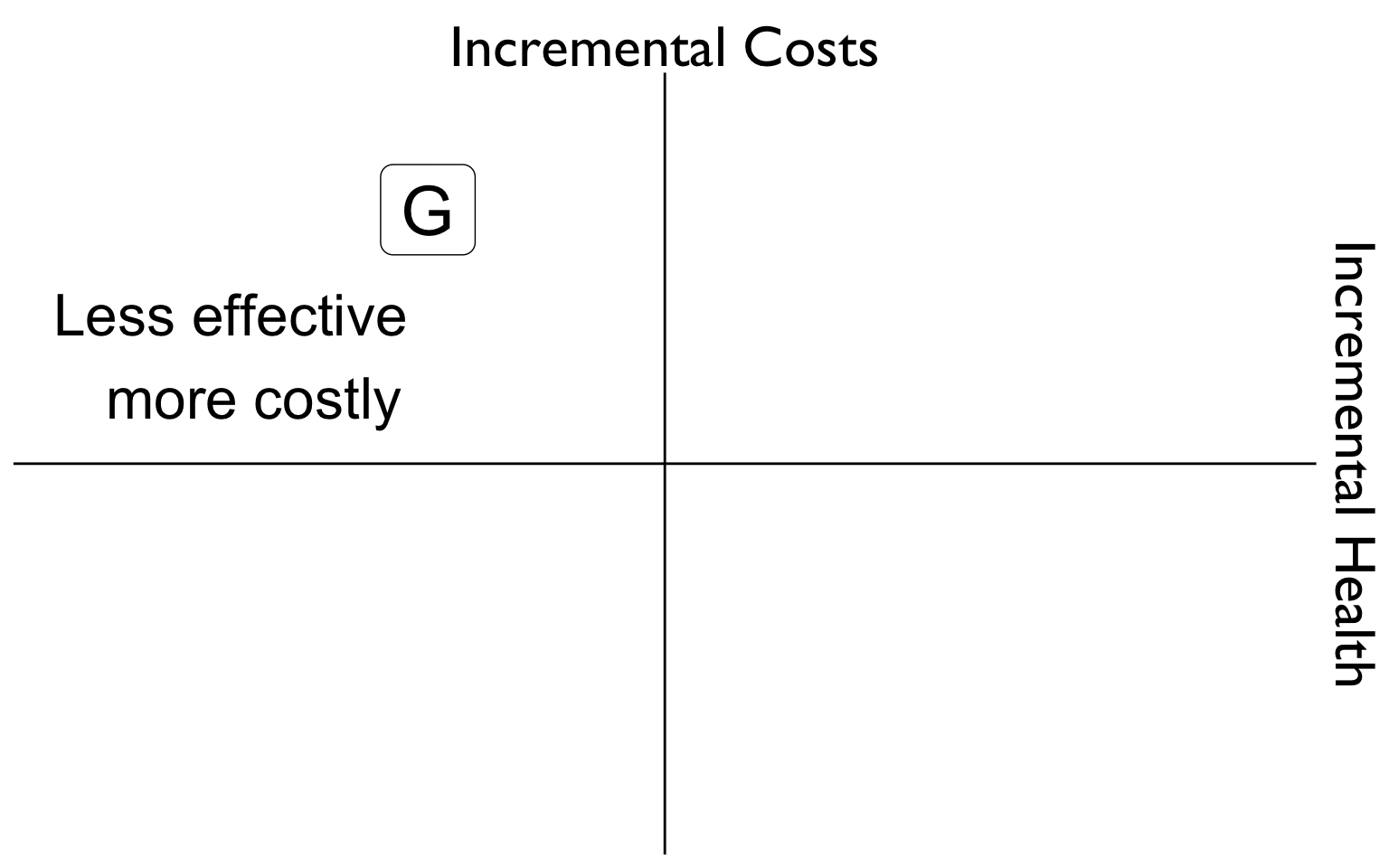
Incremental Cost-Effectiveness Analysis

Learning Objectives and Outline

Learning Objectives

• Differentiate between average & incremental CEA ratios

• Characterize decision problems by whether they are competing or non-competing

• Compute and interpret ICERs

• Practice ruling out “dominated” and “extendedly dominated” strategies

• Identify “high-value” versus “low value” care strategies, based on generally accepted cost-effectiveness thresholds

Outline

1. Review of CEA ratio
2. Non-competing versus competing CEAs
3. Incremental CEA

4. Dominance & extended dominance
5. Comparators
6. CEA thresholds

Cost-Effectiveness Analysis

Cost-Effectiveness Analysis

• Quantifies how to maximize the quality & quantity of life from among competing alternatives, given restricted resources

• It’s an explicit measure of value for money

• A POPULATION-LEVEL decision-making tool

Cost-Effectiveness Analysis IS NOT

• Indiscriminate cost-cutting
• Downsizing
• For individual-level decision making
• The only tool for decision-making

Cost-Effectiveness Analysis

Cost of Intervention

Cost of Alternative

Benefit of Intervention

Benefit of Alternative

Cost-Effectiveness Analysis

Cost of Intervention

Cost of Alternative

Benefit of Intervention

Benefit of Alternative

Cost-Effectiveness Ratio

Cost of Intervention

\quad - \quad

Cost of Alternative

\frac{\quad \quad \quad \quad \quad \quad \quad \quad \quad \quad \quad \quad \quad \quad \quad \quad}{\quad \quad \quad \quad \quad \quad \quad \quad \quad \quad \quad \quad \quad \quad \quad \quad}

Benefit of Intervention

\quad - \quad

Benefit of Alternative

Cost-Effectiveness Ratio

C_1

\quad - \quad

C_0

\frac{\quad \quad \quad \quad \quad \quad \quad \quad \quad \quad \quad \quad \quad \quad \quad \quad}{\quad \quad \quad \quad \quad \quad \quad \quad \quad \quad \quad \quad \quad \quad \quad \quad}

E_0

\quad - \quad

E_1

Cost-Effectiveness Ratio

\Delta C

\frac{\quad \quad \quad \quad }{\quad \quad \quad \quad \quad }

\Delta E

Incremental Cost-Effectiveness Ratio

Most often used, since for most conditions there is already some available treatment.

• C_1: net present value of total lifetime costs of new treatment
• C_0: net present value of total lifetime costs of default treatment
• E_1: effectiveness of new treatment, measured in expected life expectancy, quality-adjusted life years (QALYs) or disability-adjusted life years (DALYs), or some decision-relevant health outcome.
• E_0: effectiveness of default treatment

\frac{C_1 - C_0 \quad (\Delta C)}{E_1 - E_0 \quad (\Delta E)}

Neurologic Disease Decision Tree

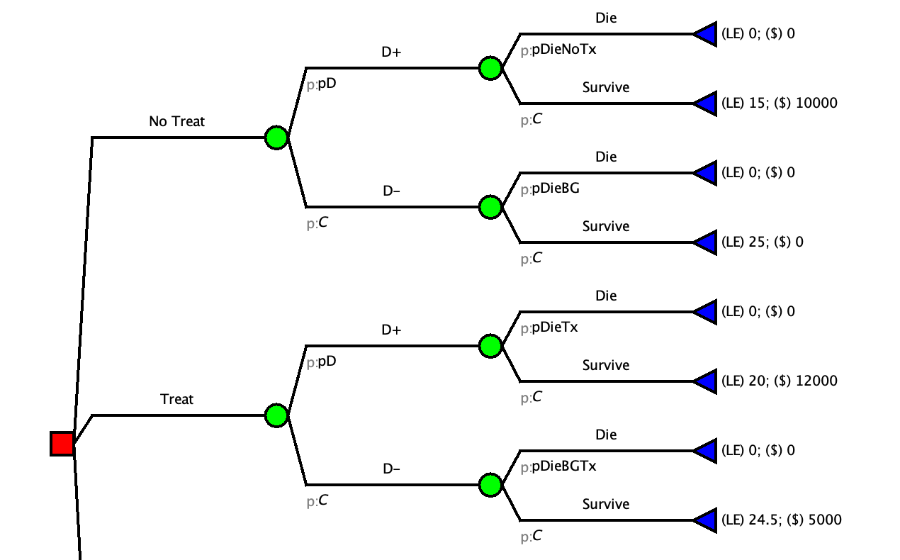
Outcomes

• C_{treat} = expected cost of treat everyone strategy.
• C_{no treat} = expected cost of treat no one strategy.
• C_{biopsy} = expected cost of biopsy strategy.

Outcomes

• C_{treat} = expected cost of treat everyone strategy.
• C_{no treat} = expected cost of treat no one strategy.
• C_{biopsy} = expected cost of biopsy strategy.
• E_{treat} = expected life expectancy of treat everyone strategy.
• E_{no treat} = expected expectancy of treat no one strategy.
• E_{biopsy} = expected expectancy of biopsy strategy.

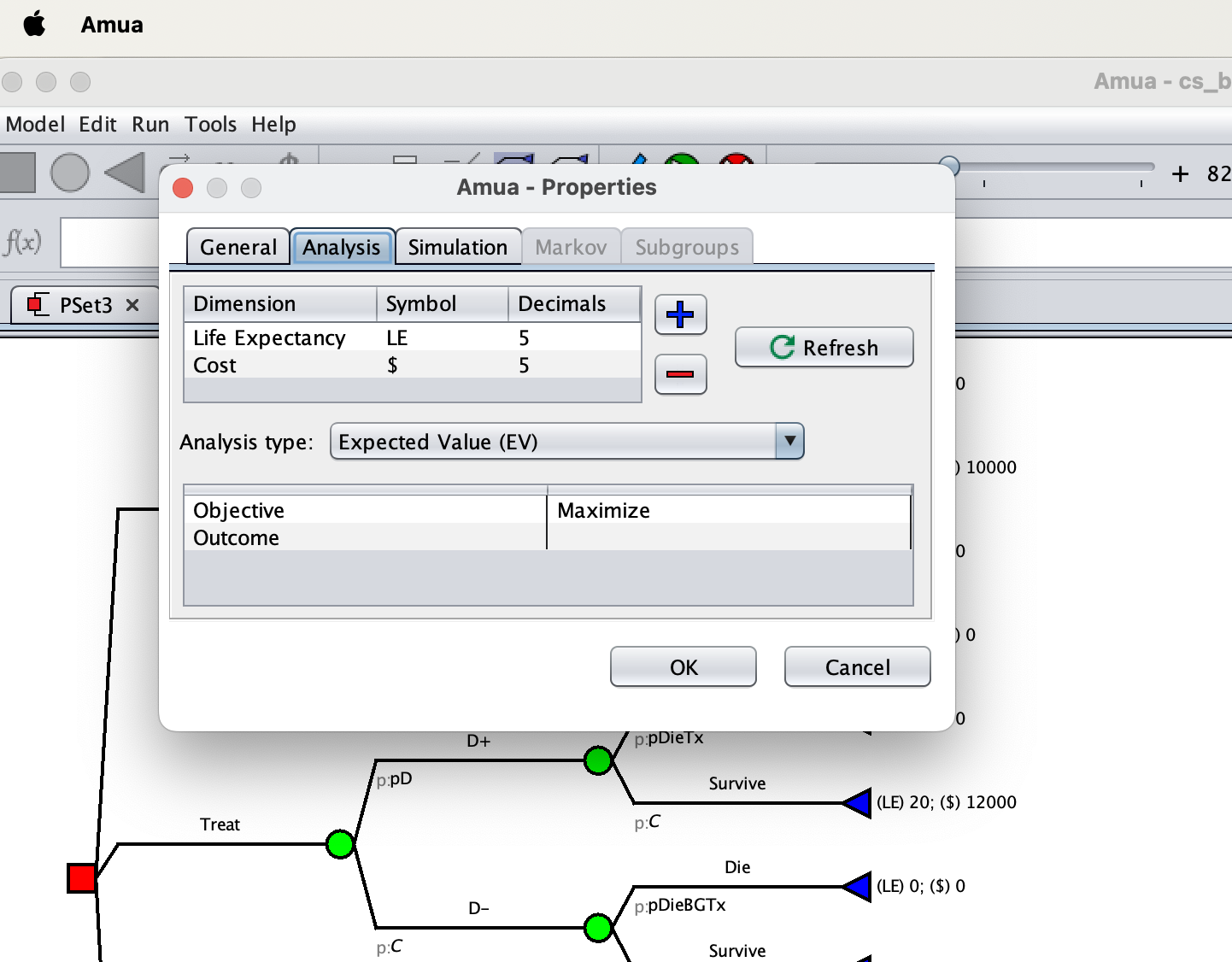
Outcomes in Amua

Treat All vs. Treat None

Strategy: Treat No One

Treat All vs. Treat None

Strategy: Treat All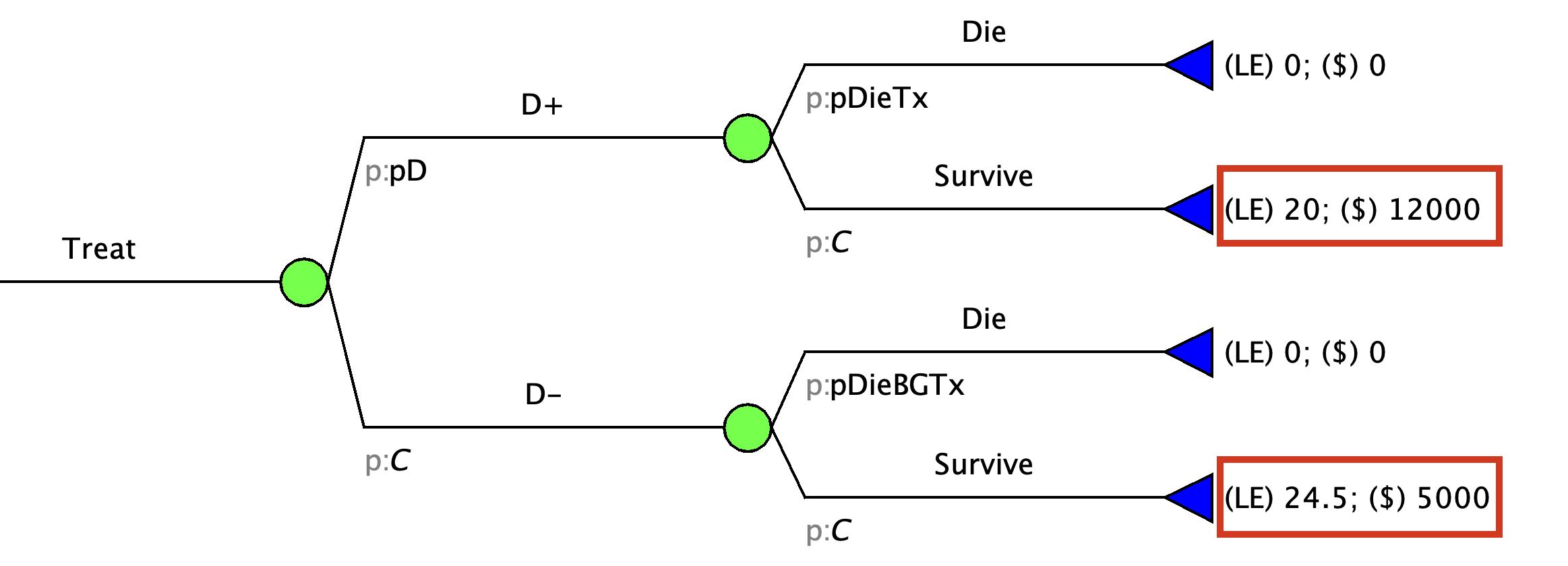

Key Takeaways (For Now)

• Treatment yields higher life expectancy for those with disease, but comes at a cost.
• Treatment yields lower life expectancy for those without the disease, and also comes at a cost.
• Biopsy can help balance these two outcomes by better targeting treatment, but also comes with costs and risks.
• Incremental CEA provides a transparent framework for quantifying and weighing these considerations.

Average Cost-Effectiveness Ratio

Special case where C_0 and E_0 are assumed to be zero.

• C_1: net present value of total lifetime costs of new treatment
• C_0: Assumed zero
• E_1: effectiveness of new treatment, measured in expected life expectancy, quality-adjusted life years (QALYs) or disability-adjusted life years (DALYs), or some decision-relevant health outcome.
• E_0: Assumed zero

\begin{aligned} ICER &= \frac{C_1 - 0}{E_1 - 0} \\ &= \frac{C_1}{E_1 } \end{aligned}

Non-Competing vs. Competing CEAs

Use of CEA in two situations

1. Shopping Spree: Decision problem has non-competing programs/interventions.

• Each program is compared to a null alternative; therefore, you’re calculating an “average” cost-effectiveness ratio.

Use of CEA in two situations

2. Competing Choice: Decision problem has competing programs/interventions for the same purpose; these choices are mutually exclusive.

• Two or more active alternatives in addition to the null option.
• You need to calculate an “incremental cost- effectiveness ratio”, which gives us the added cost per unit of added benefit of an option, relative to the next less expensive choice

Non-Competing (Shopping Spree) Decision Problem

How can we measure the relative priority of various health programs that compete for limited resources?

1. Cardiovascular disease program
2. Safe motherhood program
3. HIV prevention initiative
4. Child vaccination
5. Depression screening

Assumptions

• Program alternatives are assumed to be independent
• Budget constraint is only limitation
• Neither the net cost nor the net effectiveness depend on what other programs are selected
• Programs are assumed to be divisible [programs can be partially implemented]
  

Objectives: Shopping Spree Problem

Maximize the total net effectiveness (health benefit) of the programs selected.

Stay within budget.

Shopping Spree Problem

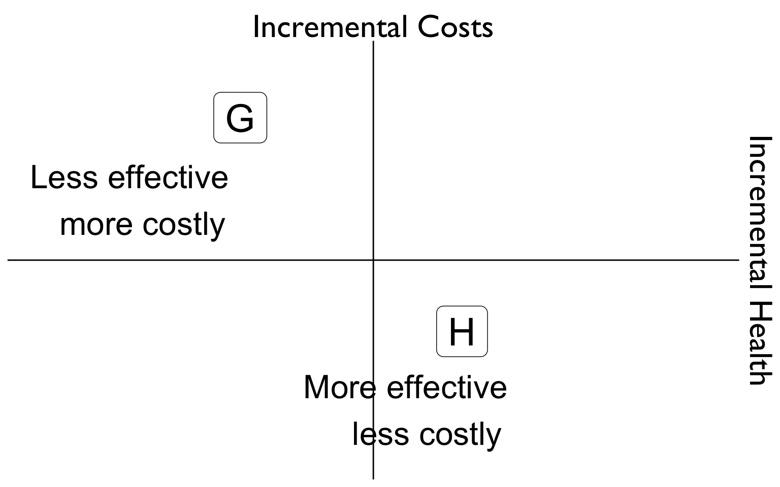
Step 1: - Rule out programs that cost $ but have negative health effects
- Dominated by alternative of “no program”

Shopping Spree Problem

Step 2:
- Select programs that are cost-saving & offer benefit; net savings can also be added to budget
- Cost-saving compared to alternative of no program

Shopping Spree Problem

Step 3:
- Rank other programs in ascending order by their cost-effectiveness ratio (lowest to highest)
- Programs are then selected from the LEAST to the MOST expensive until the budget is expended
- Final array of programs selected will depend on the budget constraint

Shopping Spree Problem

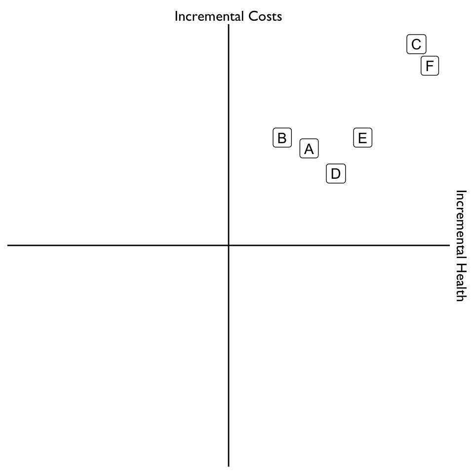
Steps 1 & 2: Rule out dominated options & select cost-saving interventions

Program	Cost	QALYs	Status
A	27	30
B	30	20
C	56	70
D	20	40
E	30	50
F	50	75
G	40	-30	Ruled Out
H	-20	20	Adopted

Shopping Spree Problem

• Initial budget: $80
• Budget savings: $20.
• Total budget: $80 + $20 = $100

Program	Cost	QALYs	Status
A	27	30
B	30	20
C	56	70
D	20	40
E	30	50
F	50	75
G	40	-30	Ruled Out
H	-20	20	Adopted

Shopping Spree Problem

• Calculate average cost-effectiveness ratio.

Program	Cost	QALYs	C/E
A	27	30	0.90
B	30	20	1.50
C	56	70	0.80
D	20	40	0.50
E	30	50	0.60
F	50	75	0.67

Shopping Spree Problem

• Calculate average cost-effectiveness ratio.
• Sort (by C/E) in ascending order .

Program	Cost	QALYs	C/E
D	20	40	0.50
E	30	50	0.60
F	50	75	0.67
C	56	70	0.80
A	27	30	0.90
B	30	20	1.50

• We want to order the RATIOS from lowest to highest for budget inclusion SINCE lower means we are gaining QALYs more efficiently – or gaining more benefit per dollar spent on care *****

Shopping Spree Problem

• Calculate cumulative costs
• Determine what is adoptable based on global budget constraint ($100)
• Calculate cumulative effects (QALYs)

Shopping Spree Problem

Budget: $100

Program	Cost	QALYs	C/E	Cumulative Cost	Cumulative QALYs
D	20	40	0.50	20	40
E	30	50	0.60	50	90
F	50	75	0.67	100	165
C	56	70	0.80	156	235
A	27	30	0.90	183	265
B	30	20	1.50	213	285

Shopping Spree Problem

Budget: $100

Program	Cost	QALYs	C/E	Cumulative Cost	Cumulative QALYs
D	20	40	0.50	20	40
E	30	50	0.60	50	90
F	50	75	0.67	100	165
C	56	70	0.80	156	235
A	27	30	0.90	183	265
B	30	20	1.50	213	285

Budget	Adopted	Effect	Threshold
100	D, E, F, H	165	0.67

1. If we have a budget of $100, then based on our program options, we could fund program D, E, & F – with a cumulative cost of $100

2. Total health benefit would include on average, 165 quality-adjusted life years gained from these programs together

3. & we might then say that our cost effectiveness threshold would be at $0.667 per QALY gained – ** this represents the point at which the budget is “optimally” allocated given budget constraints

4. More on thresholds later

Shopping Spree Problem

Budget: $150

Program	Cost	QALYs	C/E	Cumulative Cost	Cumulative QALYs
D	20	40	0.50	20	40
E	30	50	0.60	50	90
F	50	75	0.67	100	165
C	56	70	0.80	156	235
A	27	30	0.90	183	265
B	30	20	1.50	213	285

Budget	Adopted	Cost	Effect	Threshold	Remaining
150	D, E, F, H	100	165	0.67	50

Shopping Spree Problem

Budget: $150

Program	Cost	QALYs	C/E	Cumulative Cost	Cumulative QALYs
D	20	40	0.50	20	40
E	30	50	0.60	50	90
F	50	75	0.67	100	165
C	56	70	0.80	156	235
A	27	30	0.90	183	265
B	30	20	1.50	213	285

Budget	Adopted	Cost	Effect	Threshold	Remaining
150	D, E, F, H	100	165	0.67	50

Shopping Spree Problem

Budget: $150

Program	Cost	QALYs	C/E	Cumulative Cost	Cumulative QALYs
D	20	40	0.50	20	40
E	30	50	0.60	50	90
F	50	75	0.67	100	165
C (89.3%)	56	70	0.80	156	235
A	27	30	0.90	183	265
B	30	20	1.50	213	285

Budget	Adopted	Cost	Effect	Threshold	Remaining
150	D, E, F, C (89.3%), H	150	226.6	0.8	0

• $50 left but program C costs $56 (50/56 = 0.89)
• 0.89*70 QALYs of program C = 62.3 QALYs

Summary: Shopping Spree Problem

Maximize the total net effectiveness (health benefit)

Stay within budget

Can do the same with other objectives (e.g., Minimize costs, subject decision to ‘minimum benefit’ constraint, etc.)

Use of CEA in two situations

1. Shopping Spree: Decision problem has non-competing programs/interventions.

Use of CEA in two situations

2. Competing Choice: Decision problem has competing programs/interventions for the same purpose; these choices are mutually exclusive.

Objectives: Competing Choice Problem

Cannot implement more than one strategy at a time.

Incremental cost-effectiveness ratio is below a pre-specified adoption threshold.

What’s different?

Shopping Spree

1. Can select multiple programs
2. Different costs & effects associated with each
3. Requires calculation of an Average Cost-Effectiveness Ratio

Competing Choice

1. Programs are mutually exclusive.
2. Different costs & effects associated with each.
3. Requires calculation of an Incremental Cost-Effectiveness Ratio (ICER)

(1) Opioid pharmacotherapy is the recommended treatment for OUD in pregnancy, as we know that medication reduces the risk of overdose and relapse, improves overall retention to care, and improves pregnancy & fetal outcomes.

2. There are three classes of medications approved by the FDA – & there are several sub-modalities that are not listed here that we are modeling – such as injectable formulations versus monotherapy / etc.

3. But overall – there are options like Methadone that are full “agonists” – where the effects of the treatment increase as the dose increases

4. Buprenorphine which is a partial agonist – in other words, buprenorphine has a “ceiling effect”, so its effects can only be felt up to a certain point & then plateaus thereafter

5. And Naltrexone, which is an “antagonist” and works by blocking opioid receptors & reduces & suppresses opioid cravings

6. The difficult tradeoffs of these therapies, include:

• Access challenges & delays in care – for instance, there’s a limited # of methadone clinics across the US – there are only 3 methadone clinics in Nashville (22 total in the state) & 5 total in neighboring Mississippi

• & while buprenorphine & naltrexone, for example, can be administered in any office-based setting, methadone can only be dispensed in these specialty OTP clinics that I had mentioned earlier

• For opioid recurrence or disengagement from treatment rates, Methadone may have better outcomes BUT methadone also poses a significant risk of mortality from opioid overdose due to respiratory depression during treatment induction

• Regarding infant outcomes, buprenorphine has performed better than methadone when it comes to outcomes like preterm birth, neonatal withdrawal syndrome, & length of hospital stay, but infants exposed to Naltrexone have the least severe withdrawal overall & lowest hospital length of stay

• There are also different tradeoffs associated with treatment modalities such as tablets, film, injectables

• And then there’s many other things to consider such as inpatient versus outpatient induction periods versus continuation of care AND outcomes associated with injection versus non-injection users

7. While individuals can switch back & forth between these medications, they can only be on ONE medication at a time & we have to decide what is the best option for pregnant invidivudals with OUD given all of the tradeoffs just mentioned

Incremental CEA

1. Incremental CEA in Pictures

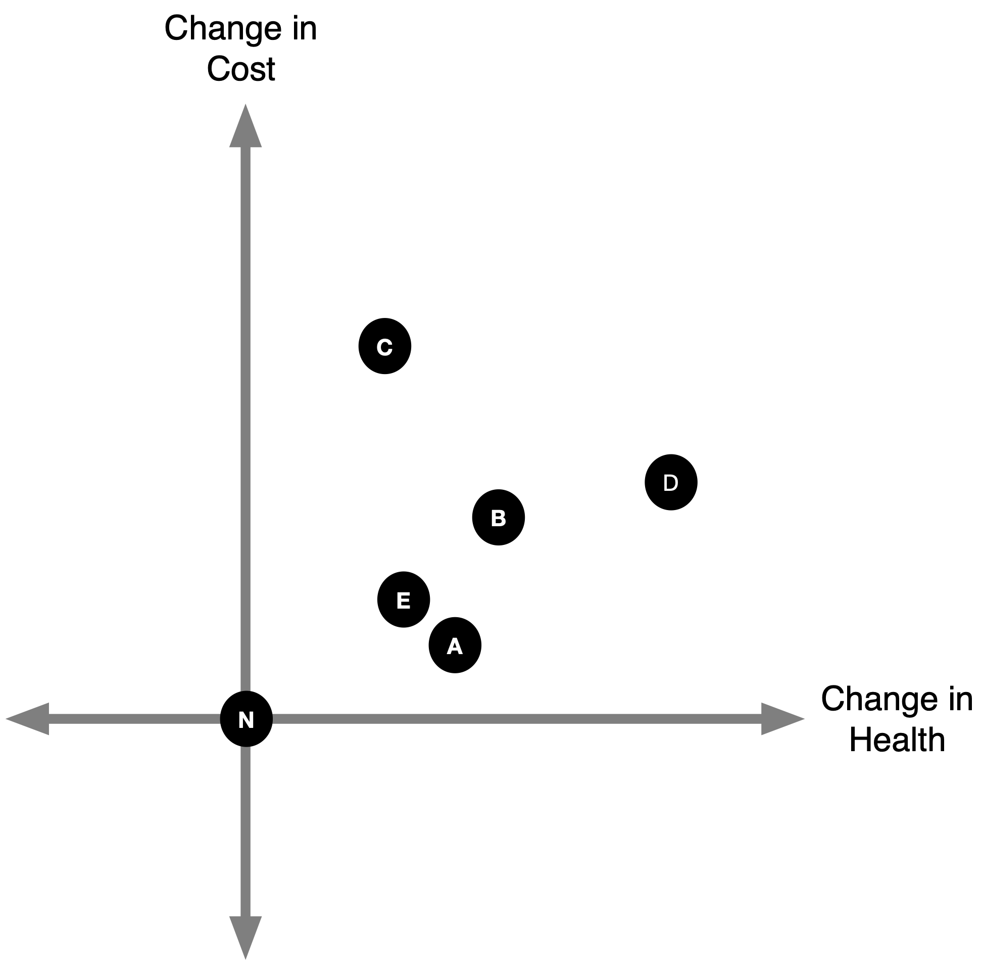
1. Calculate incremental costs and effects

• Often, a strategy capturing current practice (‘status-quo’, ‘do nothing’, ‘natural history’) is defined.
• Costs and effects are then calculated for each strategy relative to the status-quo.
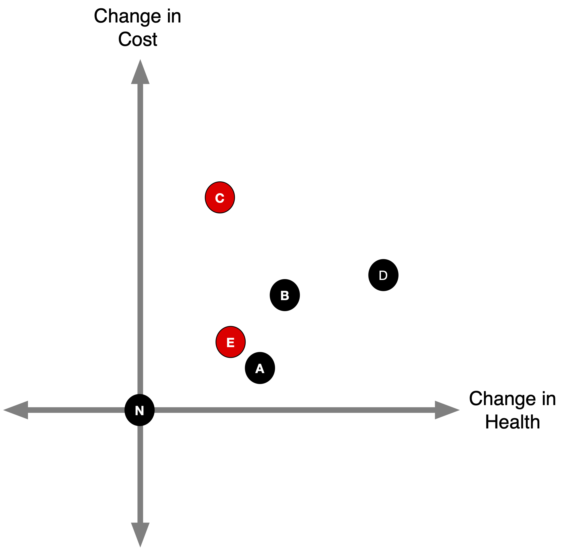
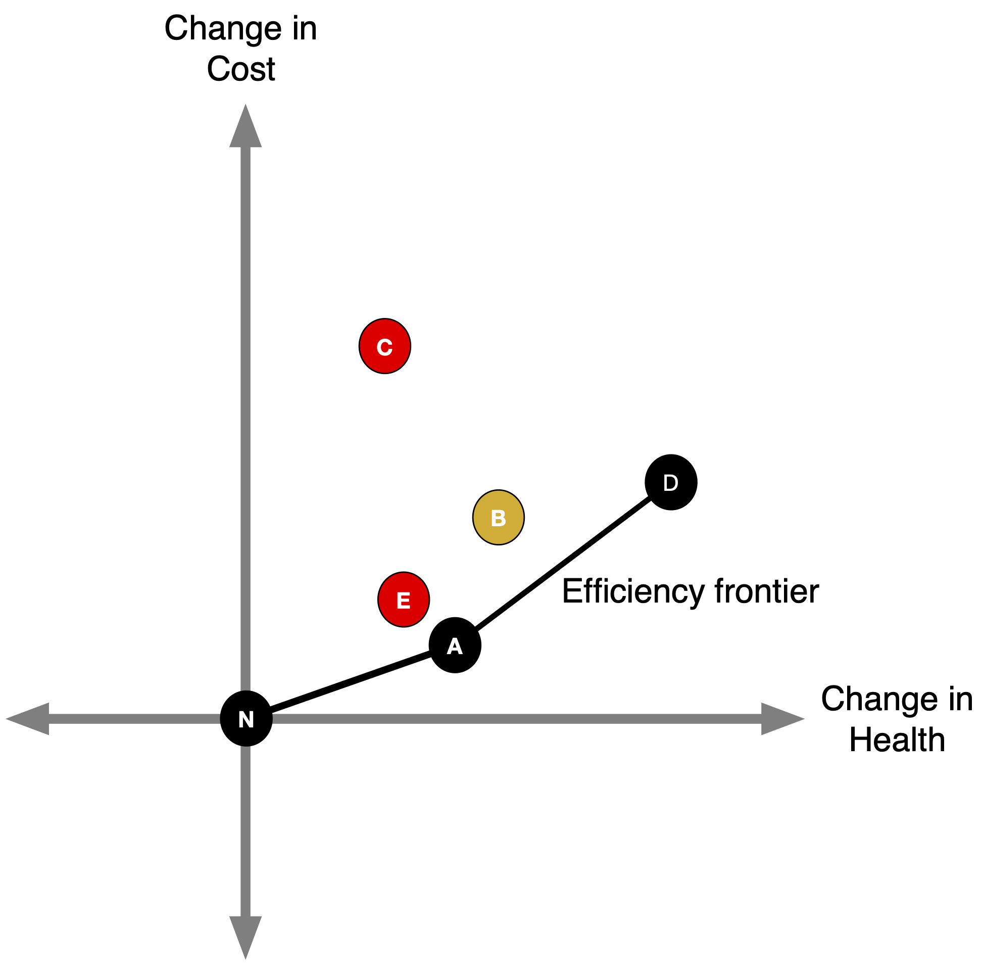
• Plot the difference in costs and effects with health effects on x-axis and cost effects on y-axis.

1. Calculate cost and effects

Identify Dominated Strategies

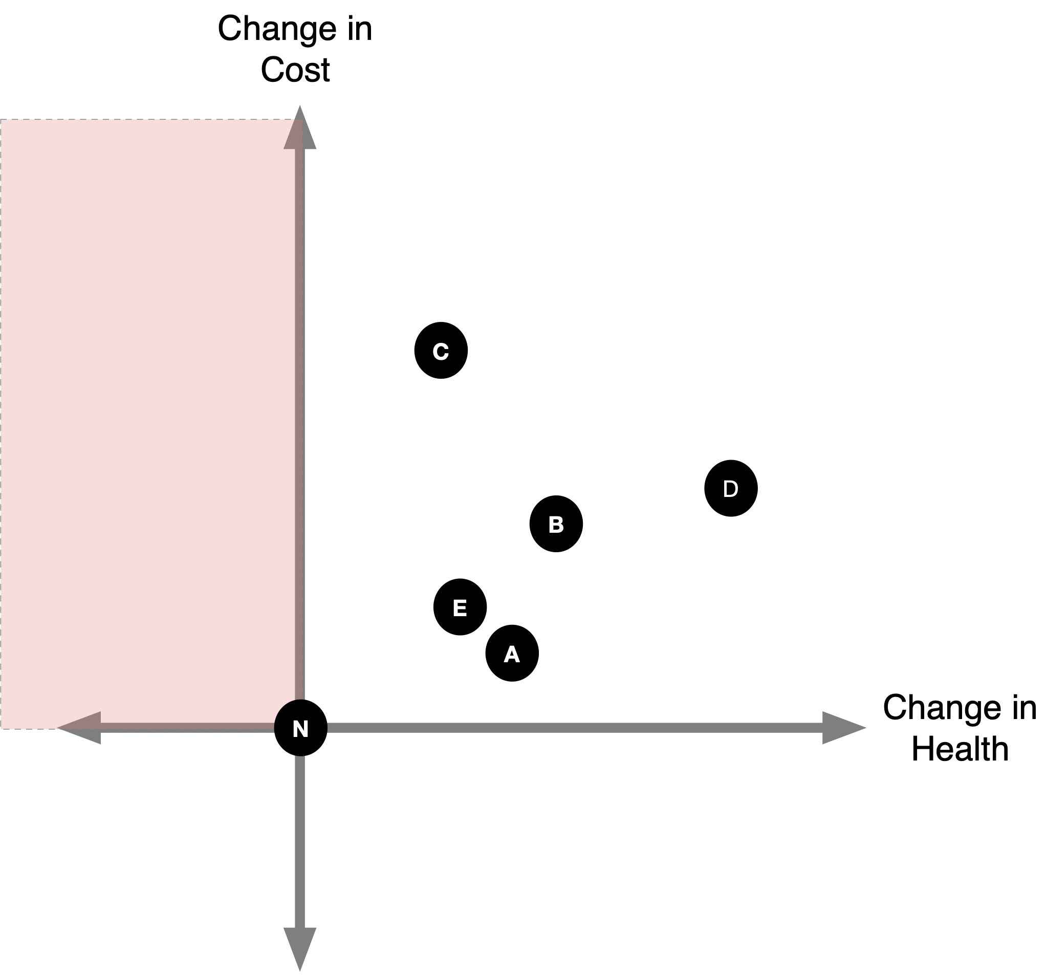
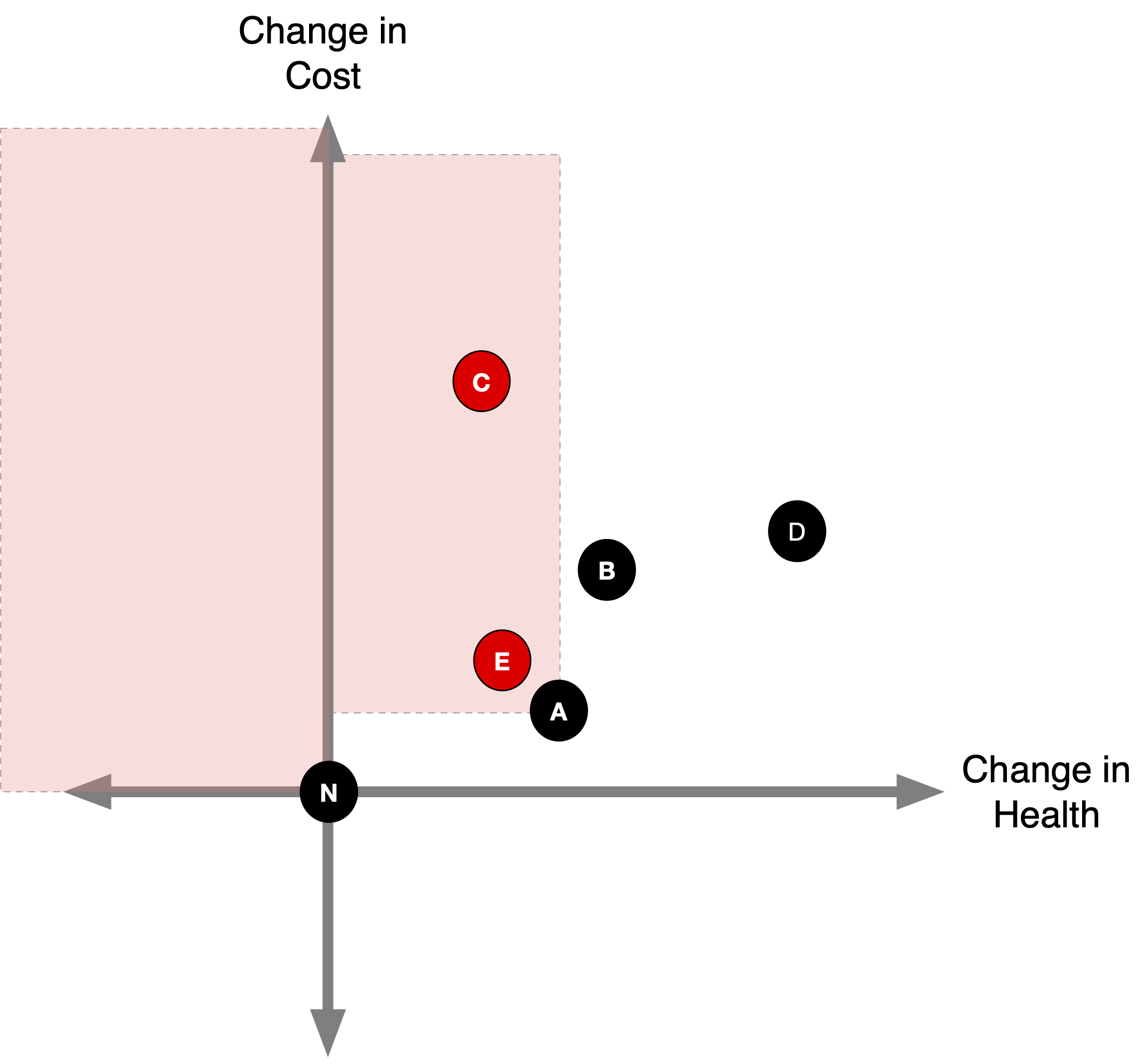
• We can rule out any strategies that result in less health at higher cost.

Identify Dominated Strategies

Identify Dominated Strategies

• We can also rule out strategies where some other competing strategy results in more (or equal) health at lower (or equal) cost.
• This is known as “strong” dominance.

Identify Dominated Strategies

Identify Dominated Strategies

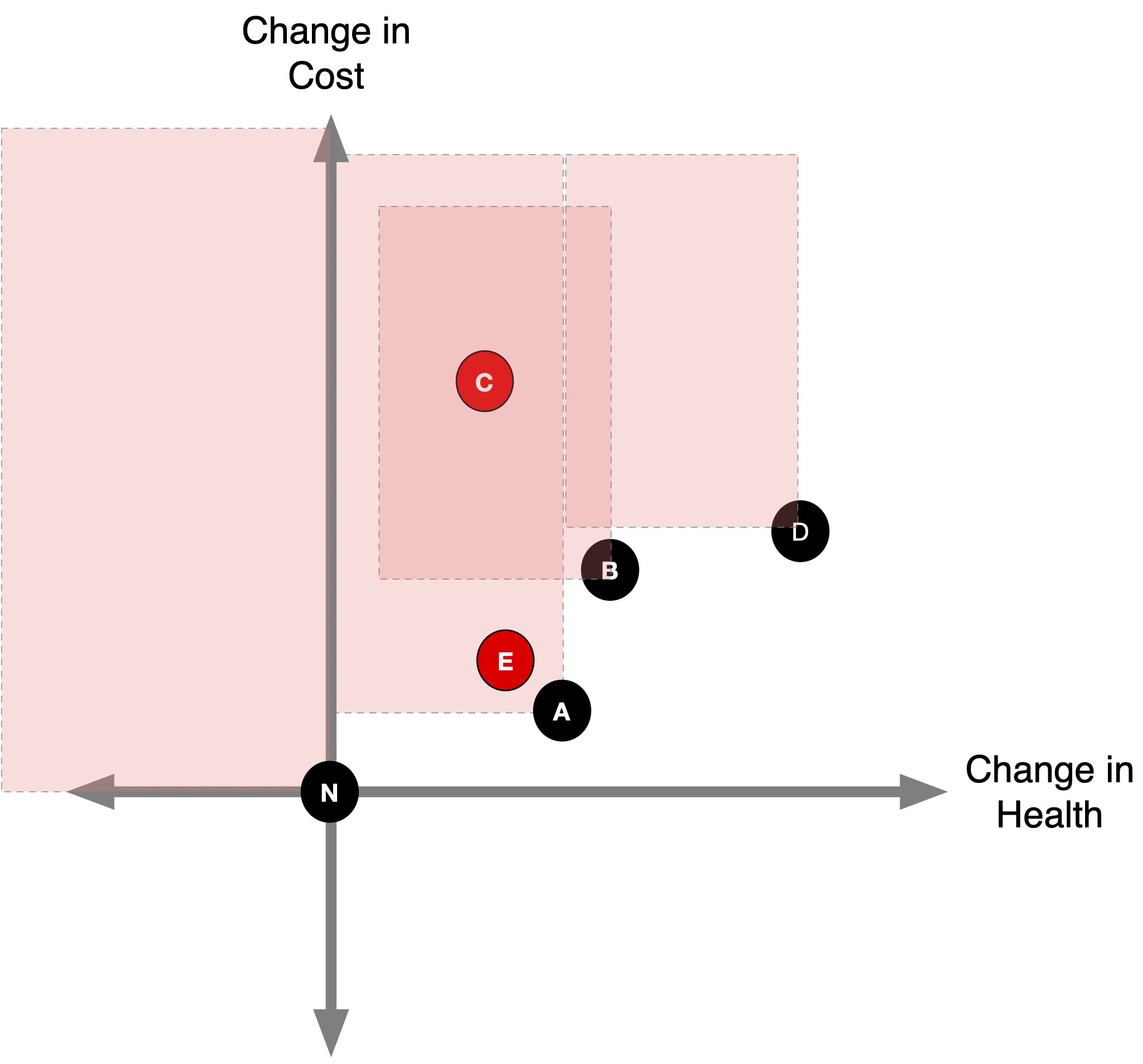
What about strategy B?

Hybrid Strategies

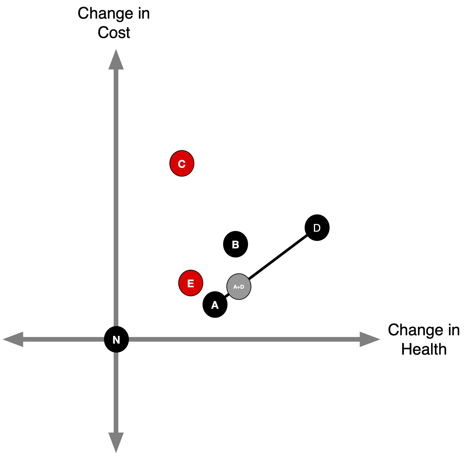
• Suppose it is feasible to partially implement strategies A and D.
  • For example, we could implement A for 90% of the population and D for 10% of the population, or vice versa.

90% A, 10% D

10% A, 90% D

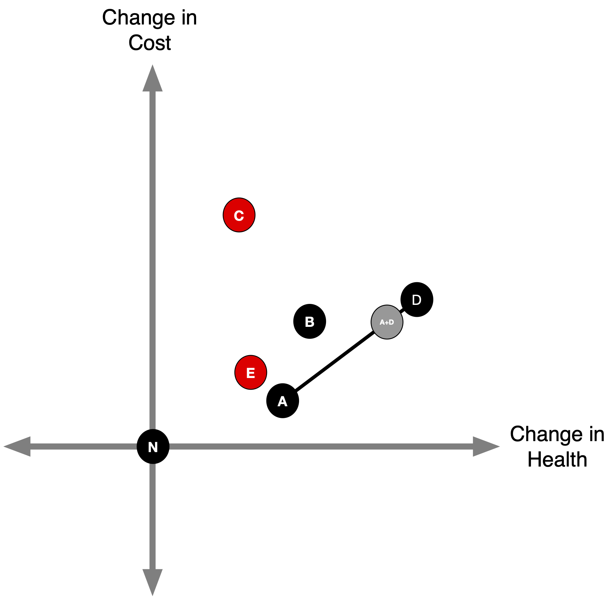
50% A, 50% D

• Can we make any statements about B now?

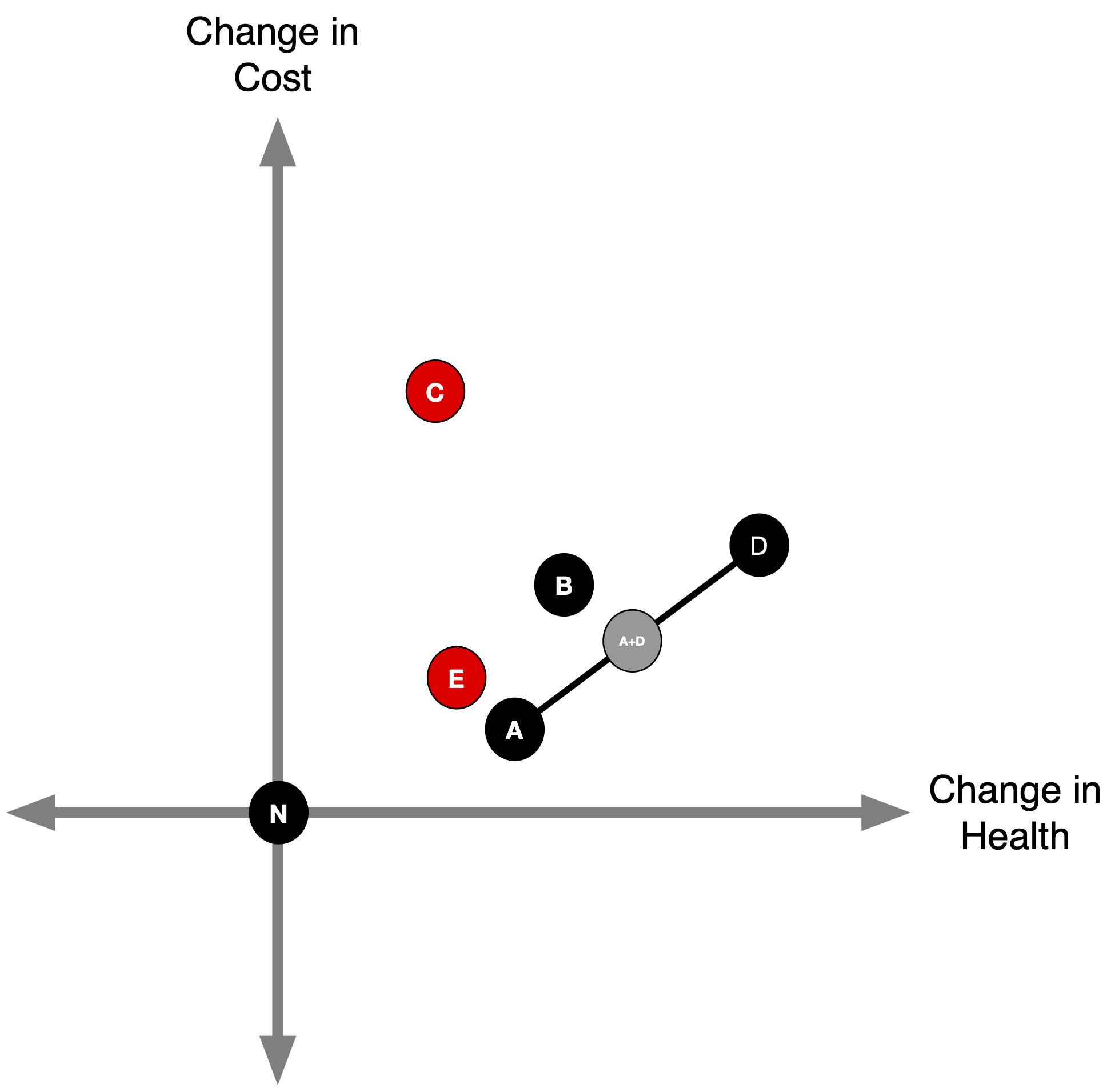
Extended (Weak) Dominance

• B is ruled out by extended (“weak”) dominance.

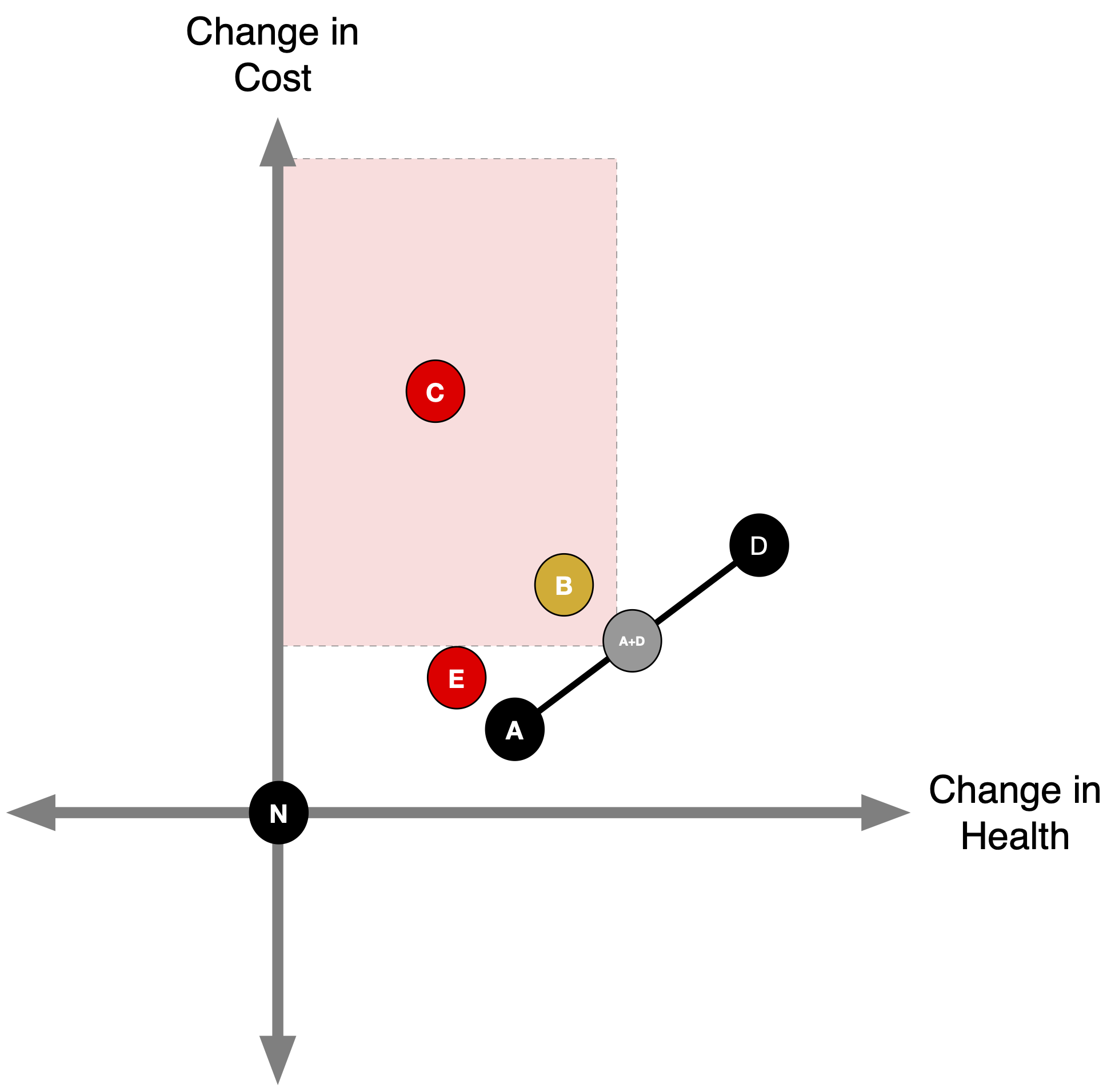
Extended (Weak) Dominance

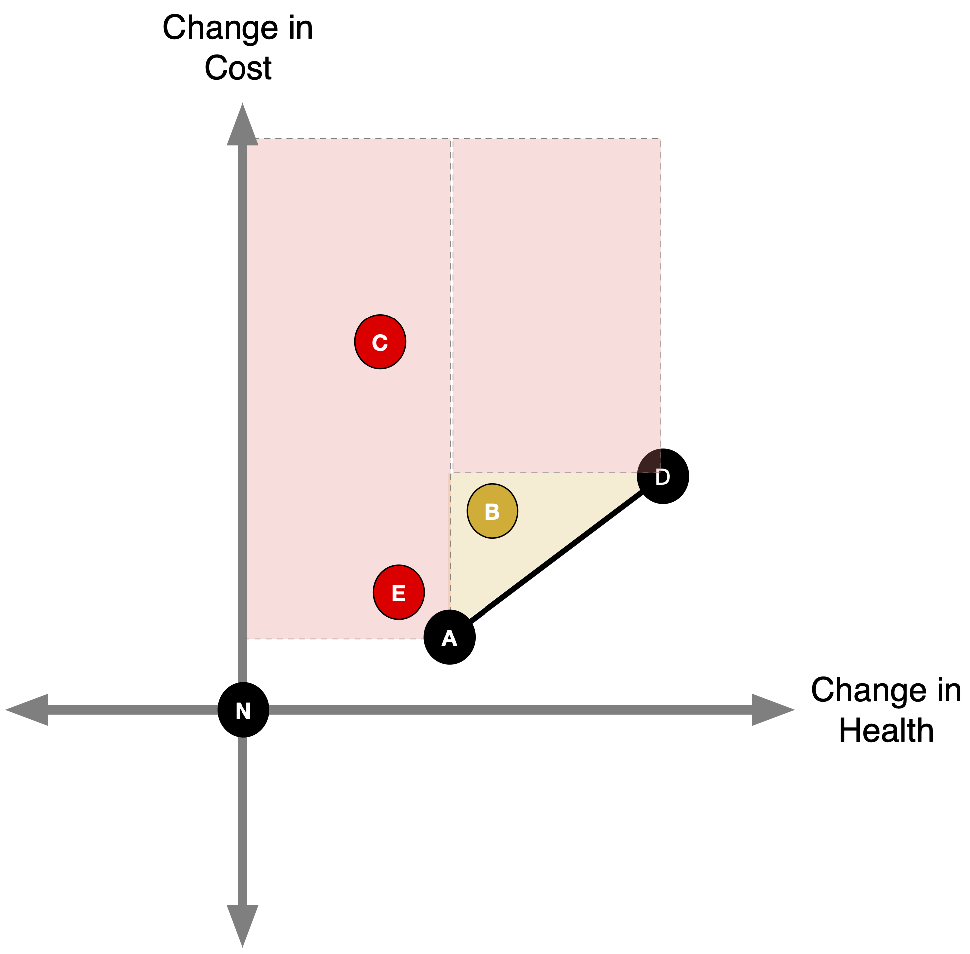
Efficiency Frontier

• The efficiency frontier is the set of non-dominated strategies.

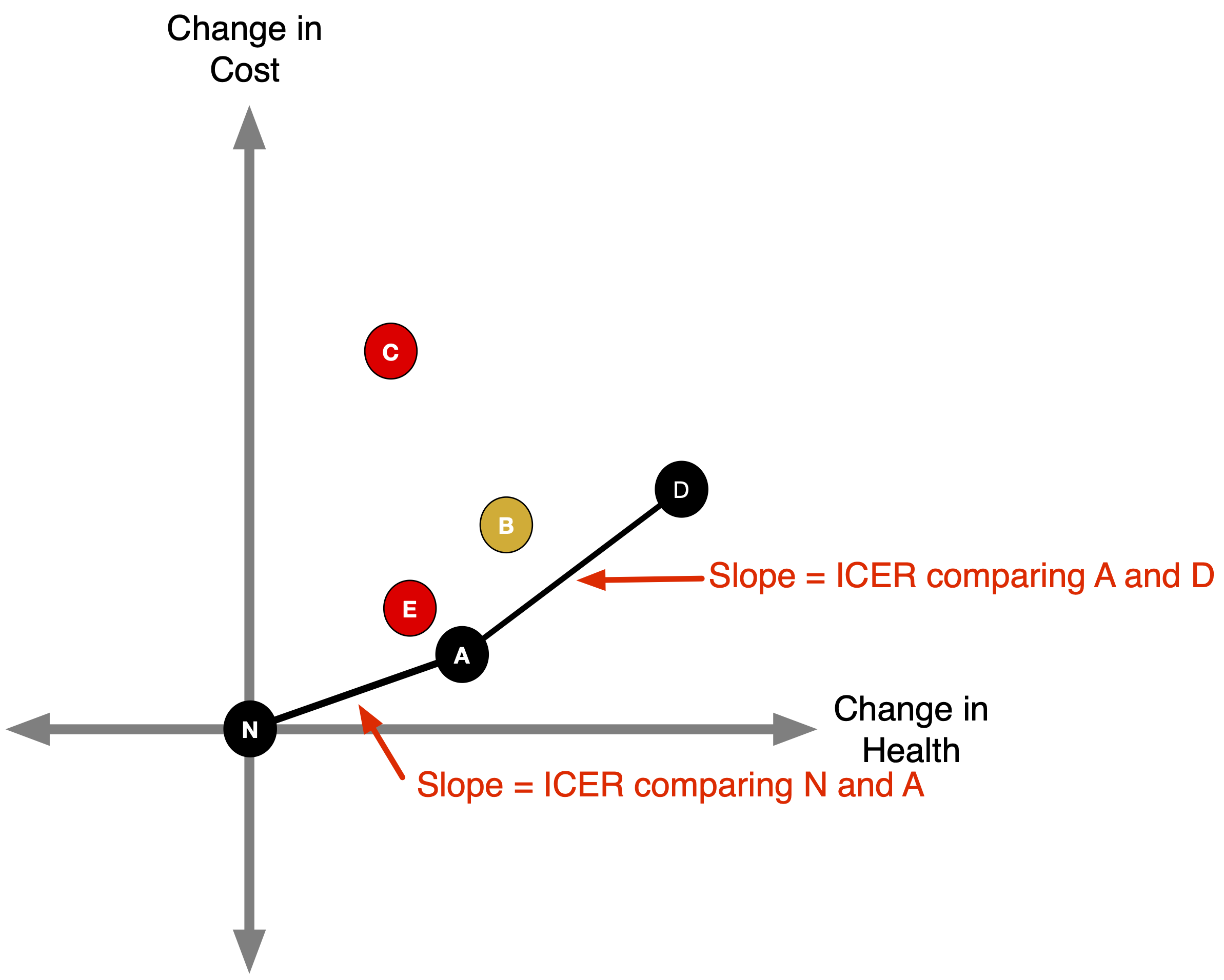
ICERs

• The slope of a line connecting two points is the incremental cost-effectiveness ratio comparing those strategies. More on this later!

2. Incremental CEA in Tables

Incremental CEA

Please note that the following example uses different strategies and values than the example used in the previous pictures!

Incremental CEA

1. Calculate costs and effects for each strategy.

2. Sort table by costs in ascending order.¹

3. Calculate ICER based on difference in costs and effects.

4. Determine dominated strategies (ICER<0).

5. Re-calculate ICERs after eliminating dominated strategies.

6. Determine strategies ruled out by extended dominance.

7. Re-calculate ICERs after ruling out all dominated strategies.

8. Repeat 5-7 as needed.

1. Least costly first, most costly last

Incremental CEA

1. Calculate costs and effects for each strategy.

Strategy	Cost	QALYs
A	16,453.99	17.332
D	24,504.08	17.491
C	33,443.25	17.580
B	21,456.58	17.409
E	43,331.68	17.491

Incremental CEA

1. Calculate costs and effects for each strategy.

2. Sort table by costs in ascending order.¹

Strategy	Cost	QALYs
A	16,454	17.332
B	21,457	17.409
D	24,504	17.491
C	33,443	17.580
E	43,332	17.491

1. Least costly first, most costly last

Incremental CEA

1. Calculate costs and effects for each strategy.

2. Sort table by costs in ascending order.¹

3. Calculate ICER based on difference in costs and effects.

Strategy	Cost	dCost	QALYs	dQALYs	ICER
A	16,454		17.332
B	21,457	5,003	17.409	0.077	64,974
D	24,504	3,048	17.491	0.082	37,171
C	33,443	8,939	17.580	0.088	101,580
E	43,332	9,888	17.491	-0.088	-112,364

1. Least costly first, most costly last

Incremental CEA

1. Calculate costs and effects for each strategy.

2. Sort table by costs in ascending order.¹

3. Calculate ICER based on difference in costs and effects.

4. Determine dominated strategies (ICER<0)

1. Least costly first, most costly last

Determining Dominated Strategies

• Let’s take a look at our table.
• Notice that strategy E has a negative ICER. Why is this?
• Strategy E raises costs but lowers QALYs.
• Therefore, we’d be better off by selecting strategy C (we would get more health gain for less money…)

Strategy	Cost	dCost	QALYs	dQALYs	ICER
A	16,454		17.332
B	21,457	5,003	17.409	0.077	64,974
D	24,504	3,048	17.491	0.082	37,171
C	33,443	8,939	17.580	0.088	101,580
E	43,332	9,888	17.491	-0.088	-112,364

Determining Dominated Strategies

• Strong dominance refers to situations where one strategy is preferred over another on both costs and health effects (e.g., QALYs).
• When we identify a strongly dominated option, we remove it from the table and re-calculate ICERS based on the remaining strategies.

Strategy	Cost	dCost	QALYs	dQALYs	ICER
A	16,454		17.332
B	21,457	5,003	17.409	0.077	64,974
D	24,504	3,048	17.491	0.082	37,171
C	33,443	8,939	17.580	0.088	101,580
E	43,332	9,888	17.491	-0.088	-112,364	Dominated

A Brief Aside on Negative ICERs

• We want to rule out strategies that cost more but result in less health.
  • This implies a negative ICER.
• But what other scenario would result in a negative ICER?
  • Strategy adds health but reduces costs.
  • This is a great strategy!

Both Strategies Have a Negative ICER

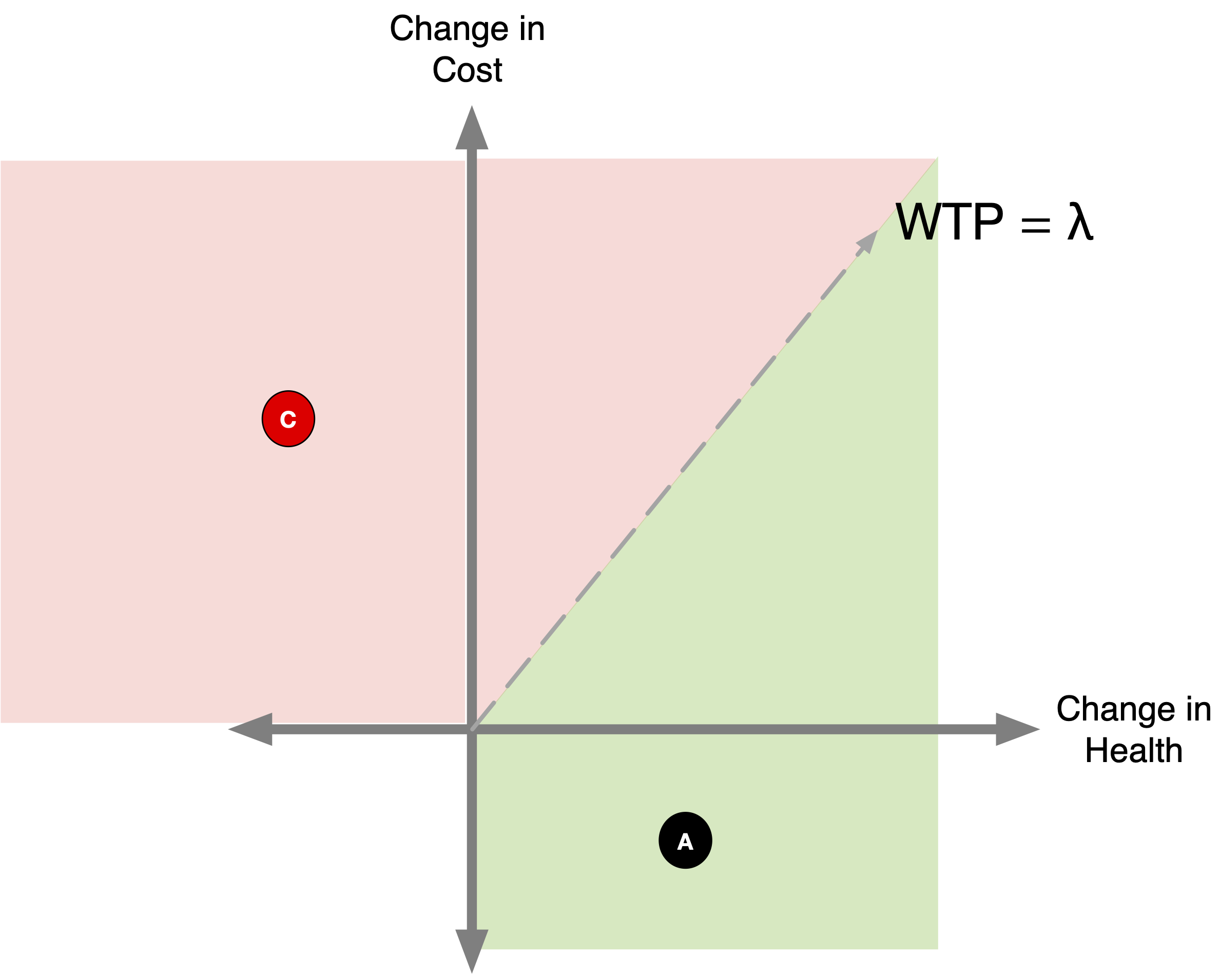
A Brief Aside on Negative ICERs

• For this reason, it is poor practice to report negative ICERs.
• Be careful when deleting a strategy becuase it has a negative ICER!
  • It may be a great strategy!

Incremental CEA

1. Calculate costs and effects for each strategy.

2. Sort table by costs in ascending order.¹

3. Calculate ICER based on difference in costs and effects.

4. Determine dominated strategies (ICER<0)

Strategy	Cost	dCost	QALYs	dQALYs	ICER
A	16,454		17.332
B	21,457	5,003	17.409	0.077	64,974
D	24,504	3,048	17.491	0.082	37,171
C	33,443	8,939	17.580	0.088	101,580
E	43,332	9,888	17.491	-0.088	-112,364	Dominated

1. Least costly first, most costly last

Incremental CEA

1. Calculate costs and effects for each strategy.

2. Sort table by costs in ascending order.¹

3. Calculate ICER based on difference in costs and effects.

4. Determine dominated strategies (ICER<0).

5. Re-calculate ICERs after eliminating dominated strategies.

Strategy	Cost	dCost	QALYs	dQALYs	ICER
A	16,454		17.332
B	21,457	5,003	17.409	0.077	64,974
D	24,504	3,048	17.491	0.082	37,171
C	33,443	8,939	17.580	0.088	101,580
E	43,332		17.491		-112,364	Dominated

1. Least costly first, most costly last

Incremental CEA

1. Calculate costs and effects for each strategy.

2. Sort table by costs in ascending order.¹

3. Calculate ICER based on difference in costs and effects.

4. Determine dominated strategies (ICER<0).

5. Re-calculate ICERs after eliminating dominated strategies.

Strategy	Cost	dCost	QALYs	dQALYs	ICER
A	16,454		17.332
B	21,457	5,003	17.409	0.077	64,974
D	24,504	3,048	17.491	0.082	37,171
C	33,443	8,939	17.580	0.088	101,580
E	43,332		17.491

1. Least costly first, most costly last

Determining Dominated Strategies

• We’re not quite done yet
• Notice something odd about strategy B?
• Its ICER is higher than the next most costly alternative (strategy D)

Strategy	Cost	dCost	QALYs	dQALYs	ICER
A	16,454		17.332
B	21,457	5,003	17.409	0.077	64,974
D	24,504	3,048	17.491	0.082	37,171
C	33,443	8,939	17.580	0.088	101,580
E	43,332		17.491

Determining Dominated Strategies

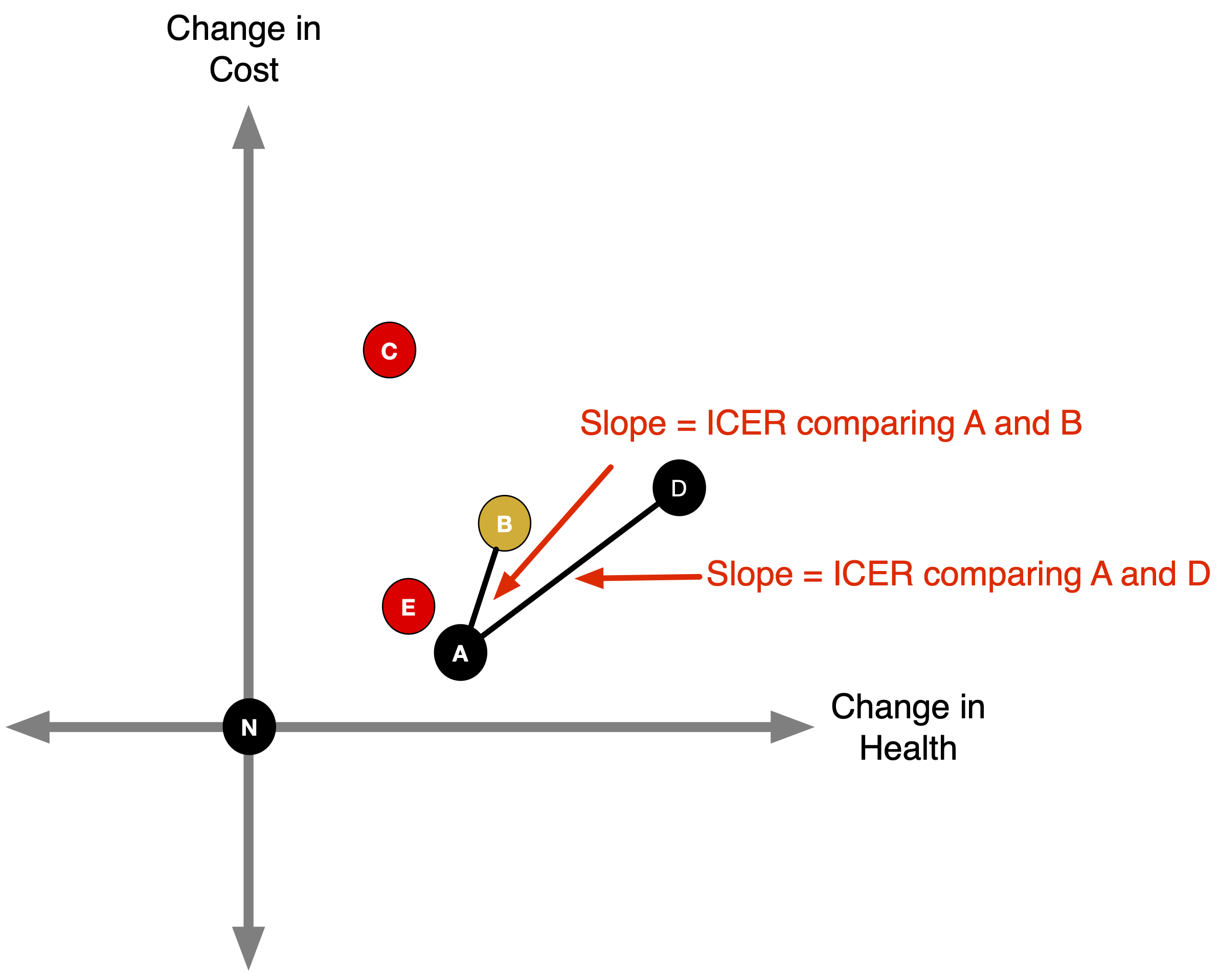
• A telltale sign of extended dominance in a (sorted) CEA table is a strategy with a higher ICER than the next most expensive option.

Strategy	Cost	dCost	QALYs	dQALYs	ICER
A	16,454		17.332
B	21,457	5,003	17.409	0.077	64,974	Dominated (Extended)
D	24,504	3,048	17.491	0.082	37,171
C	33,443	8,939	17.580	0.088	101,580
E	43,332		17.491			Dominated

Determining Dominated Strategies

• You can see this in the pictures as well ….

Incremental CEA

1. Calculate costs and effects for each strategy.

2. Sort table by costs in ascending order.¹

3. Calculate ICER based on difference in costs and effects.

4. Determine dominated strategies (ICER<0).

5. Re-calculate ICERs after eliminating dominated strategies.

6. Determine strategies ruled out by extended dominance.

Strategy	Cost	dCost	QALYs	dQALYs	ICER
A	16,454		17.332
B	21,457	5,003	17.409	0.077	64,974	Dominated (Extended)
D	24,504	3,048	17.491	0.082	37,171
C	33,443	8,939	17.580	0.088	101,580
E	43,332		17.491			Dominated

1. Least costly first, most costly last

Incremental CEA

7. Re-calculate ICERs after ruling out all dominated strategies.

Strategy	Cost	dCost	QALYs	dQALYs	ICER
A	16,454		17.332
D	24,504	8,050	17.491	0.159	50,629
C	33,443	8,939	17.580	0.088	101,580
E	43,332		17.491			Dominated
B	21,457		17.409			Dominated (Extended)

• Strategy D is more expensive than Strategy B, but Strategy D is gaining health MORE EFFICIENTLY than Strategy B

In-class practice: DALYs

Nine different prophylaxis to prevent someone with HIV from acquiring opportunistic infections related to AIDS

Strategy	Cost	DALYs
No prophylaxis	40,288	9.50
TMP-SMX	44,786	6.94
TMP-SMX, azithromycin	45,944	6.46
TMP-SMX, fluconazole	47,046	6.49
TMP-SMX, azithromycin, fluconazole	48,596	5.90
TMP-SMX, ganciclovir	54,628	6.30
TMP-SMX, azithromycin, ganciclovir	56,812	5.67
TMP-SMX, fluconazole, ganciclovir	58,082	5.70
TMP-SMX, azithromycin, fluconazole, ganciclovir	61,119	4.88

Calculate Incremental Costs and DALYs Averted

Strategy	Cost	Incremental Cost	DALYs	DALYs Averted
No prophylaxis	40,288	0	9.50	0.00
TMP-SMX	44,786	4,498	6.94	2.56
TMP-SMX, azithromycin	45,944	1,158	6.46	0.48
TMP-SMX, fluconazole	47,046	1,102	6.49	-0.03
TMP-SMX, azithromycin, fluconazole	48,596	1,550	5.90	0.59
TMP-SMX, ganciclovir	54,628	6,032	6.30	-0.40
TMP-SMX, azithromycin, ganciclovir	56,812	2,184	5.67	0.63
TMP-SMX, fluconazole, ganciclovir	58,082	1,270	5.70	-0.03
TMP-SMX, azithromycin, fluconazole, ganciclovir	61,119	3,037	4.88	0.82

Calculate incremental costs per DALY averted.

Strategy	Incremental Cost	DALYs Averted	Incremental Cost per DALY Averted
No prophylaxis	0	0.00
TMP-SMX	4,498	2.56	1,757
TMP-SMX, azithromycin	1,158	0.48	2,413
TMP-SMX, fluconazole	1,102	-0.03	-36,733
TMP-SMX, azithromycin, fluconazole	1,550	0.59	2,627
TMP-SMX, ganciclovir	6,032	-0.40	-15,080
TMP-SMX, azithromycin, ganciclovir	2,184	0.63	3,467
TMP-SMX, fluconazole, ganciclovir	1,270	-0.03	-42,333
TMP-SMX, azithromycin, fluconazole, ganciclovir	3,037	0.82	3,704

Determine dominated strategies

Strategy	Incremental Cost	DALYs Averted	Incremental Cost per DALY Averted	Status
No prophylaxis	0	0.00
TMP-SMX	4,498	2.56	1,757
TMP-SMX, azithromycin	1,158	0.48	2,413
TMP-SMX, fluconazole	1,102	-0.03	-36,733	Dominated (Strong)
TMP-SMX, azithromycin, fluconazole	1,550	0.59	2,627
TMP-SMX, ganciclovir	6,032	-0.40	-15,080	Dominated (Strong)
TMP-SMX, azithromycin, ganciclovir	2,184	0.63	3,467
TMP-SMX, fluconazole, ganciclovir	1,270	-0.03	-42,333	Dominated (Strong)
TMP-SMX, azithromycin, fluconazole, ganciclovir	3,037	0.82	3,704

Remove dominated strategies and recalculate

Determine dominated strategies

Strategy	Cost	Incremental Cost	DALYs	DALYs Averted
No prophylaxis	40,288	0	9.50	0.00
TMP-SMX	44,786	4,498	6.94	2.56
TMP-SMX, azithromycin	45,944	1,158	6.46	0.48
TMP-SMX, azithromycin, fluconazole	48,596	2,652	5.90	0.56
TMP-SMX, azithromycin, ganciclovir	56,812	8,216	5.67	0.23
TMP-SMX, azithromycin, fluconazole, ganciclovir	61,119	4,307	4.88	0.79

Determine dominated strategies

Strategy	Incremental Cost	DALYs Averted	Incremental Cost per DALY Averted	Status
No prophylaxis	0	0.00
TMP-SMX	4,498	2.56	1,757
TMP-SMX, azithromycin	1,158	0.48	2,413
TMP-SMX, azithromycin, fluconazole	2,652	0.56	4,736
TMP-SMX, azithromycin, ganciclovir	8,216	0.23	35,722	Dominated (Extended)
TMP-SMX, azithromycin, fluconazole, ganciclovir	4,307	0.79	5,452

Remove dominated strategies and recalculate

Determine dominated strategies

Determine dominated strategies

Strategy	Cost	Incremental Cost	DALYs	DALYs Averted
No prophylaxis	40,288	0	9.50	0.00
TMP-SMX	44,786	4,498	6.94	2.56
TMP-SMX, azithromycin	45,944	1,158	6.46	0.48
TMP-SMX, azithromycin, fluconazole	48,596	2,652	5.90	0.56
TMP-SMX, azithromycin, fluconazole, ganciclovir	61,119	12,523	4.88	1.02

Determine dominated strategies

Strategy	Incremental Cost	DALYs Averted	Incremental Cost per DALY Averted	Status
No prophylaxis	0	0.00
TMP-SMX	4,498	2.56	1,757
TMP-SMX, azithromycin	1,158	0.48	2,413
TMP-SMX, azithromycin, fluconazole	2,652	0.56	4,736
TMP-SMX, azithromycin, fluconazole, ganciclovir	12,523	1.02	12,277

Final Table

Strategy	Incremental Cost	DALYs Averted	Incremental Cost per DALY Averted	Status
No prophylaxis	0	0.00
TMP-SMX	4,498	2.56	1,757
TMP-SMX, azithromycin	1,158	0.48	2,413
TMP-SMX, azithromycin, fluconazole	2,652	0.56	4,736
TMP-SMX, azithromycin, fluconazole, ganciclovir	12,523	1.02	12,277
TMP-SMX, fluconazole	1,102	-0.03		Dominated (Strong)
TMP-SMX, ganciclovir	6,032	-0.40		Dominated (Strong)
TMP-SMX, fluconazole, ganciclovir	1,270	-0.03		Dominated (Strong)
TMP-SMX, azithromycin, ganciclovir	8,216	0.23		Dominated (Extended)

A note on COMPARATORS

• **The comparators are REALLY IMPORTANT
• Ideally, you want to identify ALL POSSIBLE interventions applicable to the problem, including a “do nothing” option

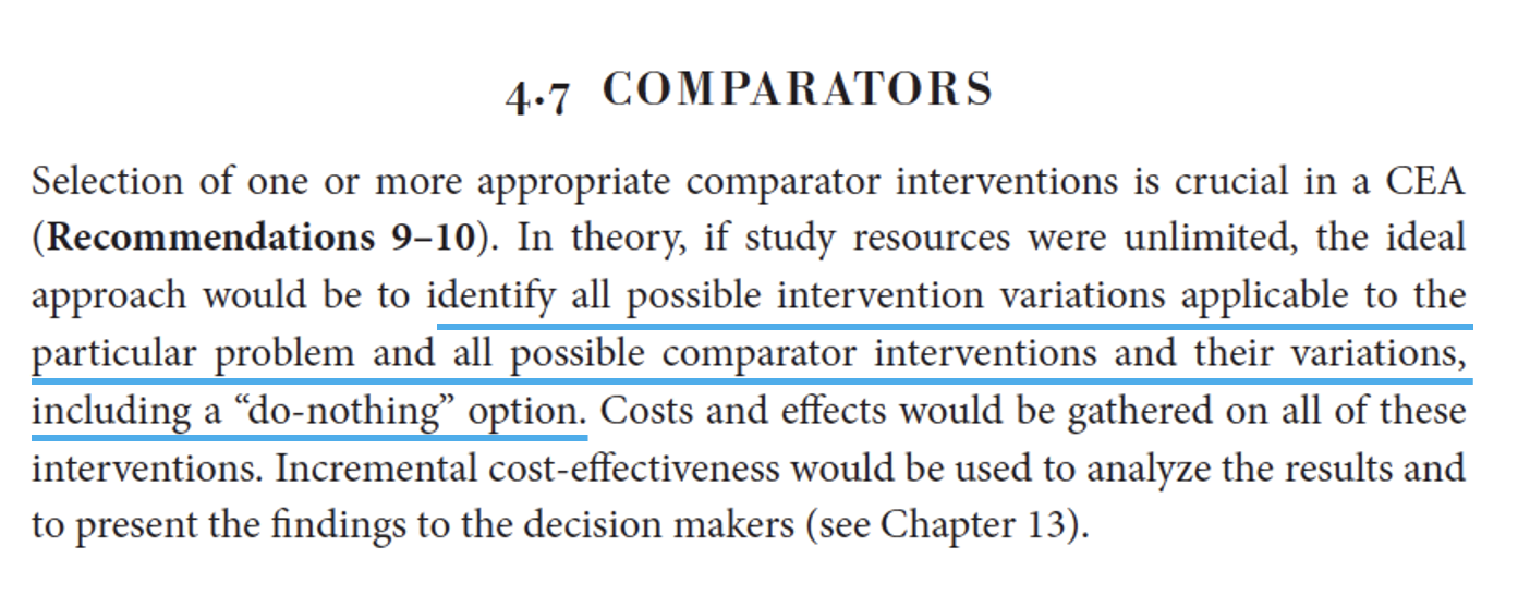
A note on COMPARATORS

• **The results can be DECEPTIVE if you decide to omit any comparators that are relevant to clinical practice

• FOR EXAMPLE, if you purposefully pick a “no treatment” comparator but leave out a closer alternative, then the analysis will grossly overstate the economic value of the drug you are assessing

• Same goes with an expensive & not very effective alternative & you leave out options that are similar in effectiveness & cost

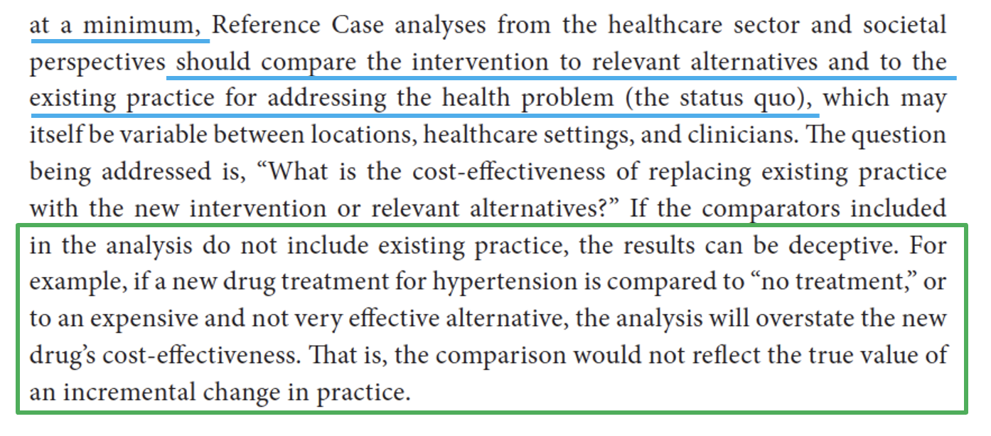
Where to draw the line?

• What CEA cannot tell us is HOW TO SPEND

CEA Thresholds

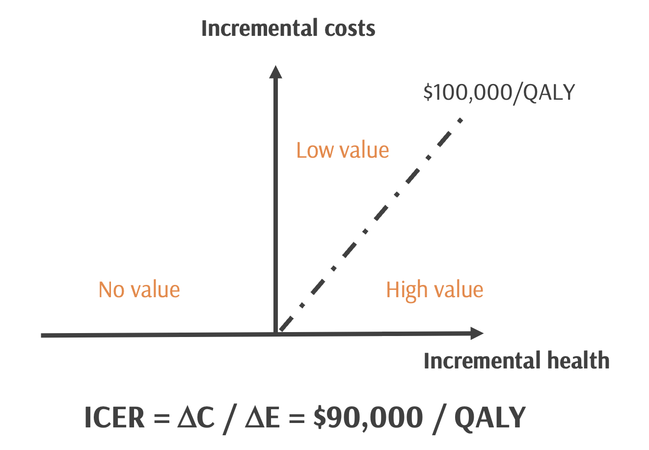
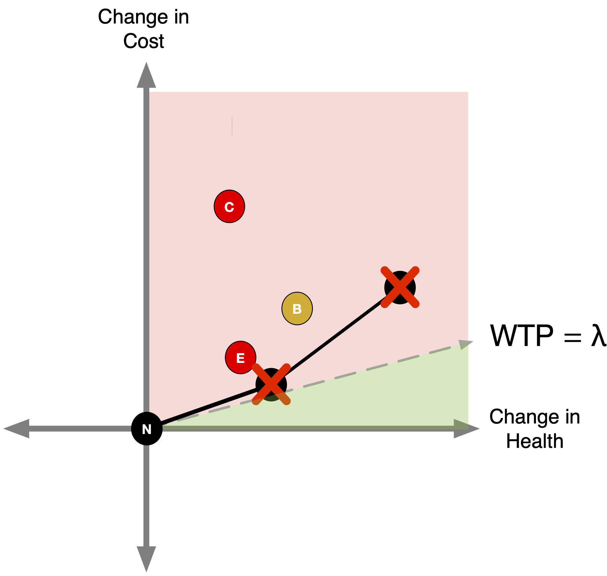
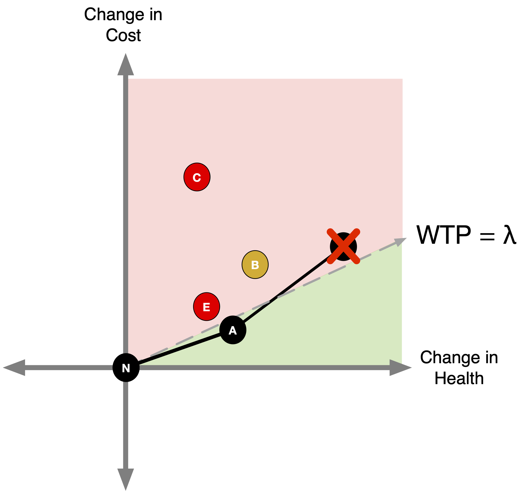
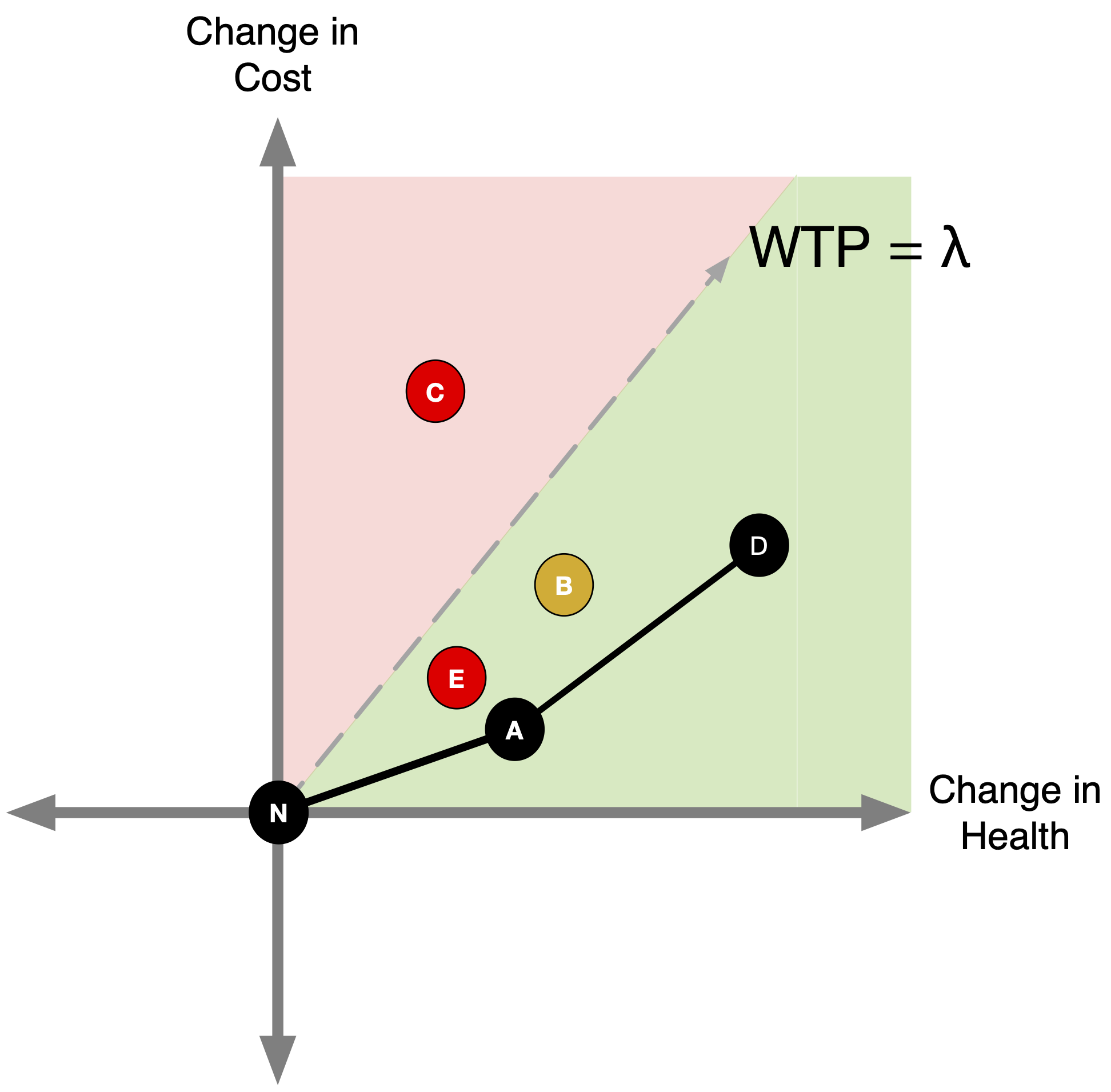
• So now we have our ICERs, but how do we make a decision?
• We must define a threshold (\lambda), or an ICER value that determines whether or not we implement a given strategy.
  • Also known as “willingness-to-pay” (WTP) threshold.

CEA Thresholds

What are common thresholds and how are they determined?

• In high income countries, common thresholds are $50,000/QALY, $100,000/QALY, and $100,000/QALY.
• In LMICs, 0.5-3x per capita gross domestic product (GDP) per DALY averted.
• More on this in a few minutes.

How do CEA Thresholds Guide Decisionmaking?

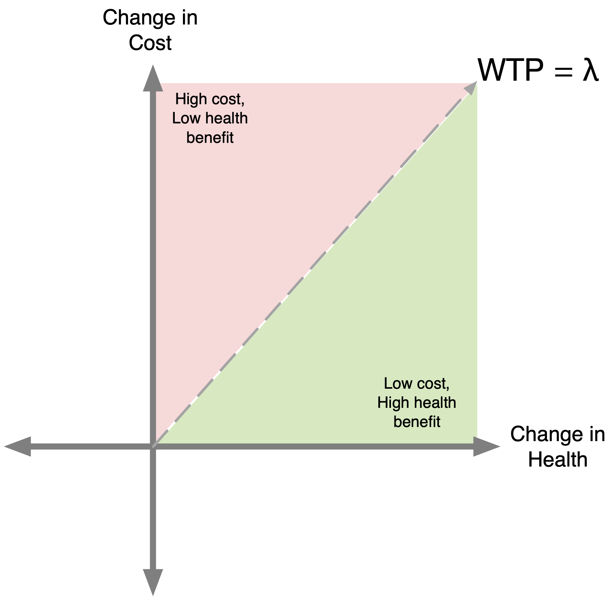
How do CEA Thresholds Guide Decisionmaking?

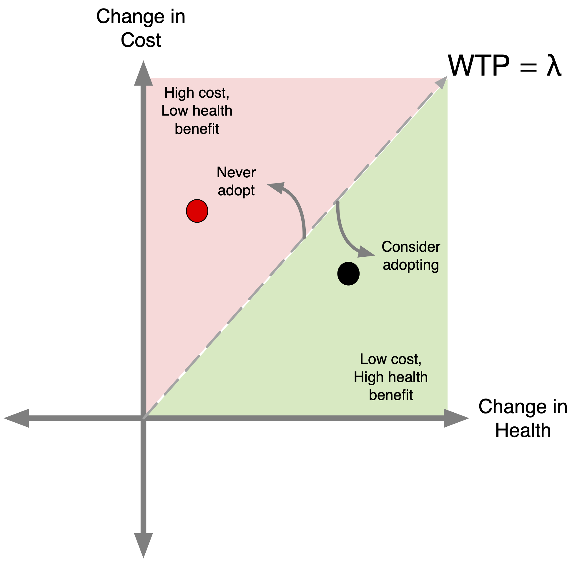
How do CEA Thresholds Guide Decisionmaking?

1. How do we know whether something is “high-value” versus “low-value” or “no-value” healthcare?

2. Let’s say we are comparing flu vaccination versus no vaccination & that our cost-effectiveness ratio yields a price per unit benefit of $90,000 / QALY gained

3. [ASK CLASS] - Would this be considered “high-value”?

4. This price must be compared to a benchmark or threshold representing either what society is willing to pay for health gains or the opportunity costs associated with displacing interventions within a fixed budget

5. In the US, the benchmark is ROUGHLY around $100,000/QALY based on willingness to pay estimates

6. A threshold’s assumed value is really important because it ultimately determines how society should invest in care, which ultimately impacts overall population health.

7. Anything above this benchmark would be considered cost-Ineffective (low value care)

8. Anything below would be considered high-value (gaining each quality-adjusted life-year at a lower cost)

9. Anything to the left is NO value care

10. This is really important because… ***Resources invested in low or no-value interventions could be better applied to more effective prevention and treatment strategies that will yield higher population health outcomes.

CEA Thresholds

CEA Thresholds

CEA Thresholds

CEA Thresholds

Different ways thresholds have been estimated: - “supply-side” (UK & Europe) - “demand-side” (US) - per capita consumption (US/LMICs)

1. There are different ways to determine a cost-effective threshold & it’s done a bit differently around the world, which we talk about in a recent paper I collaborated with UK colleagues on, which discusses the evolution of these thresholds.

2. Some countries like the UK, use what has been referred to as a “supply-side threshold” – which represents the notion of opportunity cost – whether the health generated from an adopted intervention from NICE, for instance, is greater than the health that could have been generated if the money had been spent on something else - Under a fixed budget.

3. Another way that countries like the US have defined CE thresholds is by what’s called a “demand-side” perspective, or society’s “willingness to pay” for health gains. There’s still an opportunity cost associated with this but it’s from the perspective of the goods & services we would be willing to forego for these additional health gains.

4. Similarly, another way that countries have looked at the threshold is in terms of per capita consumption - consistent with the idea that people living in countries with higher incomes are able and willing to pay more for health - which makes intuitive sense

Opportunity cost (“supply-side”)

• Decision should be informed by the value of what will be given up as a consequence of those cost.

  • Known as the “opportunity cost.”

• If resources are committed to the funding of one intervention, then they are not available to fund and deliver others (shopping spree concept)

• The opportunity cost of a commitment of resources is the health forgone because these “other” interventions that are available to the health system cannot be delivered.

• Source: See K Claxton on the estimation of the NICE threshold in the UK / Woods et al, & others

Opportunity cost (“supply-side”)

1. This is the closest to a “supply-side” CEA estimate that the US has approached
2. This simulation looked at the Opportunity Cost attributed to persons dropping health insurance due to health insurance premium increases (which often happens when intervention costs are very high – it’s often the consumers that bear the burden)
3. The authors found that the threshold should be around $100,000/QALY gained (which is typically what we use in the US)
4. But UK academics would argue that this isn’t a true opportunity cost estimate because it doesn’t evaluate the opportunity cost of displacing interventions for other more effective (but often more costly) alternatives –

• either within the health care sector or displacing other programs in other sectors because of how much we spend on health care
• & there’s many other things to consider such as effect of increasing healthcare costs on patient copays, wait times, generosity of employer plans, or on public insurance

Opportunity cost (“supply-side”)

If you don’t consider the budget under which you are operating, then some medications could take up half the budget and displace interventions that produce significant health gain OR in the US, could increase premiums or take away $$ from other sectors

Academics have argued that the threshold should be lower/on the more conservative end for higher priced therapies (NICE uses a budget impact threshold of 20,000 GBP/QALY for these higher priced therapies as opposed to 30,000 GBP/QALY for others)

Willingness to pay (“demand-side”)

1. Given that our health system is more complicated & we don’t necessarily have a “fixed” budget, per se, the US has largely defined thresholds based on what is often referred to as “demand-side” or “willingness-to-pay” criteria, which can also be represented as the willingness to forego other types of consumption to improve one’s health.

2. This willingness to pay has been derived through surveys & also what Medicare has been willing to pay for interventions

3. Some have argued that understanding a population’s willingness to pay is important, especially in a single-payer system that is funded through social insurance – ensuring that individuals have a role in decision-making

4. But there is huge variation in willingness to pay studies - varied substantially by condition, especially those for extending or saving life (higher WTP).

5. This very short perspective piece gives an overview of the thresholds we have used in the US in the past & what they are largely based on (has largely been arbitrary) – it’s 2 pages & would recommend reading

CEA Thresholds in LMICs

1. Other thresholds that countries have used are based on per capita GDP; mainly the threshold of 1-3X per capita GDP

2. Although this threshold range roughly corresponds to what has become convention for high-income countries (1X per capita GDP in the US is around $60,000 & 3 times that is the upper end of what we use – typically use 50,000 as lower end, 100,000 as the base, and 150,000 as an upper end)

3. BUT per capita consumption in wealthier countries exceeds the per capita consumption in low & middle-income countries by one-to-two orders of magnitude & therefore, some analysts have argued that healthcare spending should represent a smaller portion of per capita GDP in low to middle income countries.

CEA Thresholds in LMICs

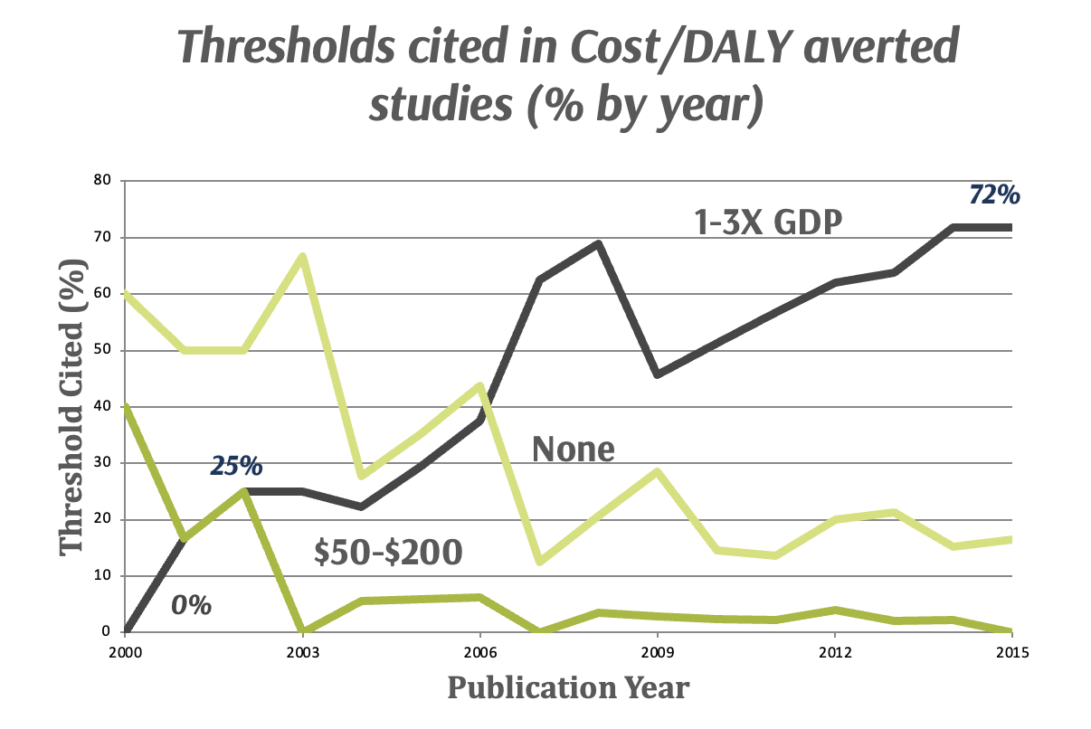
• Past WHO guidelines recommended countries use following guidelines: An intervention is cost-effective if cost/DALY averted is less than 1-3X per capita GDP of country
• Some have argued the WHO’s guidelines may be too high and result in adoption of interventions that displace existing services that provide greater health benefit.
• Suggest 0.5 GDPpc is a more appropriate benchmark for low-income countries and 0.71 GDPpc for middle-income countries (see Woods et al 2016)

1. Analysts have also argued that the threshold should be lower for these countries based on a healthcare budget perspective

2. In Peru, for example, a study found that the addition of one breast cancer treatment could be cost-effective under the broad 1-3X per capita GDP criteria; however, the cost of adding the new drug would exceed Peru’s entire budget for breast cancer treatment.

CEA Thresholds in LMICs

1. You can see from my paper on this –

2. We found:

• The proportion of PUBLISHED studies citing a threshold of 1-3X per capita GDP has increased over time & this largely corresponds to the WHO recognition of this threshold in the early 2000s – prior to this, most studies either cited no threshold or other CE thresholds

• The WHO has since moved away from recommended this threshold since it has received A LOT of backlash, including from my paper

3. Until we come up with a better measure, the DSP3 & other academics have estimated more conservative thresholds (previous slide) that I would use for LMICs & would NOT use the per capita assumptions

4. But we still don’t have a perfect threshold estimate

HIV Example From Earlier

Strategy	Incremental Cost	DALYs Averted	Incremental Cost per DALY Averted	Status
No prophylaxis	0	0.00
TMP-SMX	4,498	2.56	1,757
TMP-SMX, azithromycin	1,158	0.48	2,413
TMP-SMX, azithromycin, fluconazole	2,652	0.56	4,736
TMP-SMX, azithromycin, fluconazole, ganciclovir	12,523	1.02	12,277
TMP-SMX, fluconazole	1,102	-0.03		Dominated (Strong)
TMP-SMX, ganciclovir	6,032	-0.40		Dominated (Strong)
TMP-SMX, fluconazole, ganciclovir	1,270	-0.03		Dominated (Strong)
TMP-SMX, azithromycin, ganciclovir	8,216	0.23		Dominated (Extended)

HIV Example from Earlier

• If our CE threshold was 2x GDP (GDP = $2,500), which option would we choose as decision makers?
• If our CE threshold was 1x GDP (GDP = $2,500), which option would we choose as decision makers?

Next: ICER Case Study