Using Simulation to Calculate Power and Minimum Detectable Effects

This posting will walk through the steps to perform power and minimum detectable effect calculations via simulation.

library(mcreplicate)
library(tidyverse)
library(tictoc)
library(CVXR)

Define the Data Generation Process

params <-
    list(
        n = 100,
        p = 1,
        beta = 0
    )

Now we define the data generation process formula:

dgp <- function(params) {
    with(params,{
        X <- matrix(rnorm(n * p), nrow=n)
        colnames(X) <- paste0("beta_", beta)
        Y <- X %*% beta + rnorm(n)
        data.frame(Y,X)
    })
}

Define the Estimator

est <- function(df) {
    Y <- df[,"Y"]
    X <- as.matrix(df[,setdiff(colnames(df),"Y")])
    ls.model <- lm(Y ~ 0 + X)   # There is no intercept in our model above
    m <- data.frame(ls.est = coef(ls.model))
    rownames(m) <- gsub("Xbeta","beta",rownames(m))
    m <- cbind(m,confint(ls.model))
    m
}

Define the discrimination function

• Reject if 0 is within the 95% confidence interval.
• Accept is 1 minus the above.

disc <- function(fit) {
    beta.hat <- fit["X",]
    accept <- 1-as.integer(dplyr::between(0,beta.hat[,2],beta.hat[,3]))
    return(accept)
}

est_power <- function(params) {
    cat(params$beta)
    cat("\n")
    params %>%  
      dgp() %>%  
        est() %>% 
          disc()

}

Results

Power

B = 1000
power =
    seq(100,1000,100) %>%
    map(~(mc_replicate(B,est_power(modifyList(params,list(beta = .1,n=.x))),mc.cores=10))) %>%
    map_dbl(~(mean(.x)))  %>%
    data.frame(row.names = seq(100,1000,100)) %>%
    rownames_to_column(var = "N") %>%
    set_names(c("N","power")) %>%
    as_tibble() %>%
    mutate(N = as.numeric(paste0(N)))

power %>% knitr::kable()

N	power
100	0.151
200	0.298
300	0.407
400	0.510
500	0.612
600	0.695
700	0.748
800	0.805
900	0.865
1000	0.885

power %>%
    ggplot(aes(x = N , y = power)) + geom_line() +
    ggthemes::theme_few()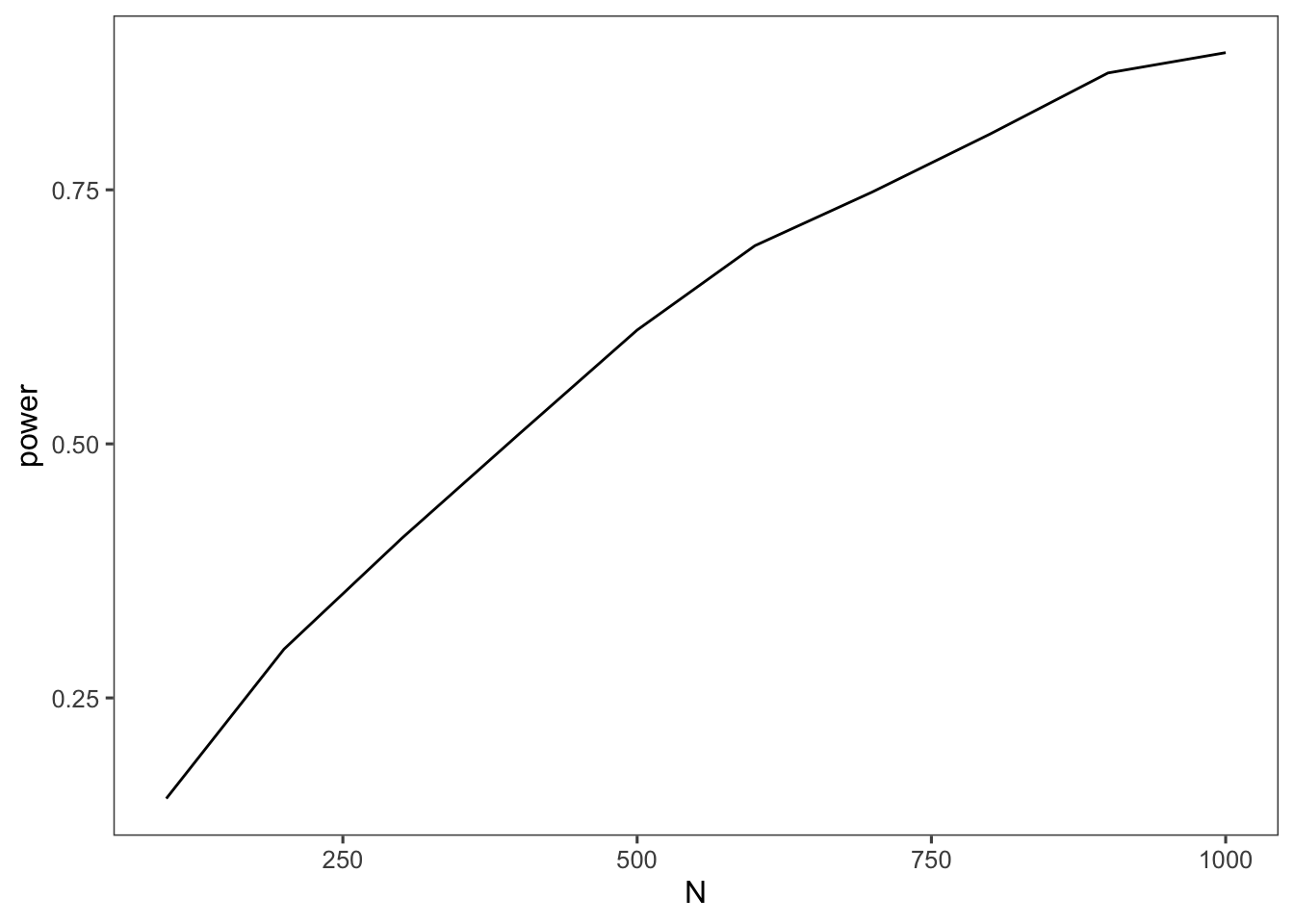

Minimum Detectable Effects

calc_mde <- function(.x, B=10000) {
    power <- mc_replicate(B,est_power(modifyList(params,list(beta = .x,n=1000))),mc.cores=10) %>% mean()
    abs(power-.8)
}

search_grid <- seq(0,.1,0.01)
mde =
    search_grid %>%
    map(~(mc_replicate(B,est_power(modifyList(params,list(beta = .x,n=1000))),mc.cores=10))) %>%
    map_dbl(~(mean(.x)))  %>%
    data.frame(row.names = search_grid) %>%
    rownames_to_column(var = "N") %>%
    set_names(c("beta","power")) %>%
    as_tibble() %>%
    mutate(beta = as.numeric(paste0(beta)))

mde %>%
    ggplot(aes(x = beta, y = power)) + geom_line() +
    ggthemes::theme_few() +
    ylim(c(0,1)) + geom_hline(aes(yintercept =0.8),lty=2)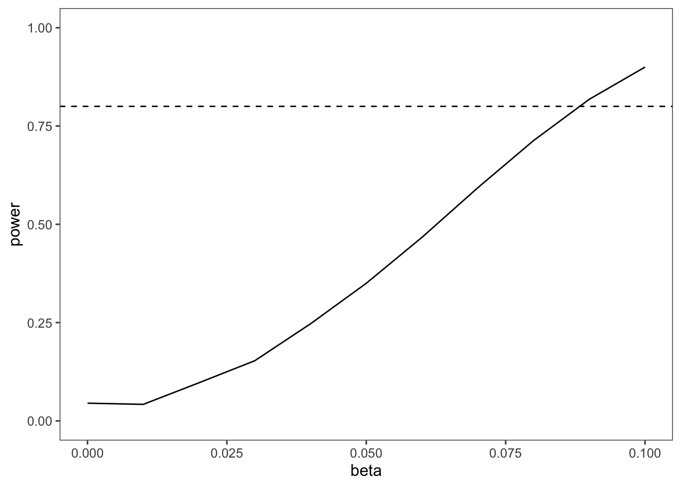

closest <- mde$beta[which(abs(mde$power-.8)==min(abs(mde$power-.8)))]
closest

[1] 0.09